9. [DocR] Textual User Interface for ADAO (TUI/API)
This section presents advanced usage of the ADAO module using its text
programming interface (API/TUI). This interface gives user ability to create a
calculation object in a similar way than the case building obtained through the
graphical interface (GUI). A scripted form of a case built in the GUI can be
obtained directly using the TUI export button  integrated in the
interface, but more complicated or integrated cases can be build only using TUI
approach. When one wants to elaborate directly the TUI calculation case, it is
recommended to extensively use all the ADAO module documentation, and to go
back if necessary to the graphical interface (GUI), to get all the elements
allowing to correctly set the commands. The general used notions and terms are
defined in [DocT] A brief introduction to Data Assimilation and Optimization. As in the graphical interface, we point out
that the TUI approach is intended to create and manage a single calculation
case.
integrated in the
interface, but more complicated or integrated cases can be build only using TUI
approach. When one wants to elaborate directly the TUI calculation case, it is
recommended to extensively use all the ADAO module documentation, and to go
back if necessary to the graphical interface (GUI), to get all the elements
allowing to correctly set the commands. The general used notions and terms are
defined in [DocT] A brief introduction to Data Assimilation and Optimization. As in the graphical interface, we point out
that the TUI approach is intended to create and manage a single calculation
case.
9.1. Creation of ADAO TUI calculation case and examples
9.1.1. A simple setup example of an ADAO TUI calculation case
To introduce the TUI interface, lets begin by a simple but complete example of ADAO calculation case. All the data are explicitly defined inside the script in order to make the reading easier. The whole set of commands is the following one:
# -*- coding: utf-8 -*-
#
from numpy import array
from adao import adaoBuilder
case = adaoBuilder.New()
case.set( "AlgorithmParameters", Algorithm="3DVAR" )
case.set( "Background",          Vector=[0, 1, 2] )
case.set( "BackgroundError",     ScalarSparseMatrix=1.0 )
case.set( "Observation",         Vector=array([0.5, 1.5, 2.5]) )
case.set( "ObservationError",    DiagonalSparseMatrix="1 1 1" )
case.set( "ObservationOperator", Matrix="1 0 0;0 2 0;0 0 3" )
case.set( "Observer",            Variable="Analysis", Template="ValuePrinter" )
case.execute()
The result of running these commands in SALOME (either as a SALOME “shell” command, in the SALOME Python command window of the interface, or by the script execution entry of the menu) is the following:
Analysis [0.25000264 0.79999797 0.94999939]
9.1.2. Detailed setup of an ADAO TUI calculation case
More details are given here on the successive steps of the setup of an ADAO TUI
calculation case. The commands themselves are detailed just after in the
Set of available commands in text user interface TUI. We keep the indication [...] of preceding
or following lines to emphasize that these commands can be inserted in the
middle of a complete stream of Python scripting for a real study.
The creation and initialization of a study are done using the following
commands, the case object name of the ADAO TUI calculation case being let
free to the user choice:
[...]
from numpy import array
from adao import adaoBuilder
case = adaoBuilder.New()
[...]
It is recommended to import by default the numpy module or some of its
embedded constructors such as the array one, to make easier its upcoming
use in the commands.
Thereafter, the case has to be build by preparing and storing the data that
define the study. The commands order does not matter, it is sufficient that all
the concepts, required by the algorithm used, are present. The user can refer
to the [DocR] Reference description of the ADAO commands and keywords and its sub-parts to get details about commands
by algorithm. Here, we define successively the chosen data assimilation or
optimization algorithm and its parameters, then the a priori state
 (named
 Background) and its errors covariance
 (named
 BackgroundError), and after that, the observation
 (named
 Observation) and its errors covariance
 (named
 ObservationError):
[...]
case.set( 'AlgorithmParameters', Algorithm='3DVAR' )
#
case.set( 'Background',          Vector=[0, 1, 2] )
case.set( 'BackgroundError',     ScalarSparseMatrix=1.0 )
#
case.set( 'Observation',         Vector=array([0.5, 1.5, 2.5]) )
case.set( 'ObservationError',    DiagonalSparseMatrix='1 1 1' )
[...]
As a remark, vector or matrix inputs can be given as objects of type str,
list or tuple of Python, or of type array or matrix of Numpy.
For these last two cases, one has only to import Numpy module before.
After that, one has to define the operators  of observation and
possibly
of observation and
possibly  of evolution. In all cases, linear or non-linear, they can
be defined as functions. In the simple case of a linear operator, one can also
define it using the matrix that corresponds to the linear operator. In the most
simple present case of a linear operator, we use the following syntax for an
operator from
of evolution. In all cases, linear or non-linear, they can
be defined as functions. In the simple case of a linear operator, one can also
define it using the matrix that corresponds to the linear operator. In the most
simple present case of a linear operator, we use the following syntax for an
operator from  into itself:
[...]
case.set( 'ObservationOperator', Matrix = "1 0 0;0 2 0;0 0 3")
[...]
In the most frequent case of a non-linear operator of  into
into
 , it has to be previously available as a Python function,
known in the current name space, which takes a Numpy vector (or an ordered
list) of size
, it has to be previously available as a Python function,
known in the current name space, which takes a Numpy vector (or an ordered
list) of size  as input and which returns as output a Numpy vector
of size
as input and which returns as output a Numpy vector
of size  . When the non-linear operator is the only one to be defined
by the keyword “OneFunction”, its adjoint is directly established by
numerical calculations and it can be parametrized by the keyword
“Parameters”. The following example shows a
. When the non-linear operator is the only one to be defined
by the keyword “OneFunction”, its adjoint is directly established by
numerical calculations and it can be parametrized by the keyword
“Parameters”. The following example shows a simulation function (which
realizes here the same linear operator than above) and record it in the ADAO
case:
[...]
import numpy
def simulation(x):
    "Simulation function H to perform Y=H(X)"
    import numpy
    __x = numpy.ravel(x)
    __H = numpy.diag([1.,2.,3.])
    return numpy.dot(__H, __x)
#
case.set( 'ObservationOperator',
    OneFunction = simulation,
    Parameters  = {"DifferentialIncrement":0.01},
    )
[...]
To obtain intermediary or final results of the case, one can add some “observer”, that link a script to execute with an intermediate or final calculation variable. The reader can go the description of the way of Getting information on special variables during the ADAO calculation, and to the [DocR] Reference description of the ADAO commands and keywords in order to know what are the observable quantities. This link between an “observer” and an observable quantity is done in a similar way than the calculation data definition:
[...]
case.set( 'Observer', Variable="Analysis", Template="ValuePrinter" )
[...]
Finally, when all the required information are available in the ADAO
calculation case named case, it can be executed in a very simple way in the
environment of the Python interpreter:
[...]
case.execute()
[...]
At the end, we get a very compact script previously proposed in A simple setup example of an ADAO TUI calculation case.
9.1.3. Using more complex calculation data or information
Such an interface being written in Python, it is possible to use all the power of the language to enter more complex data than explicit declaration.
The registering of input data supports various variable types, but in addition,
these inputs can come from variables currently available in the name space of
the script. It is then easy to use previously calculated variables or obtained
by importing “user” scripts. If for example the observations are available as a
list in an external Python file named observations.py under the name
someTable, the registering of the observations in the ADAO TUI calculation
case can be done by the following operations:
[...]
from observations import someTable
case.set( 'Observation', Vector=someTable )
[...]
The first line imports the someTable variable from the external file, and
the second one register directly this table as the “Observation” data.
The simplicity of this recording demonstrates the ease of obtaining computational data from external sources, files or computing flows achievable in Python. As usual, it is recommended to the user to check its data before saving them in the ADAO TUI calculation case to avoid errors complicated to correct.
9.1.4. Obtain and use the results of calculation in a richer way
Similarly, it is possible to obtain and process the results of calculation in a richer way, following up on post-processing after the TUI calculation.
The variables of calculation results, or the internal variables coming from
optimization or data assimilation, are available through the get method of
the ADAO TUI calculation case, which send back an object of list type of the
required variable. The reader can go to the Variables and information available at the output
for a detailed description on this subject.
For instance, we give some script lines that allow to get the number of iterations of the optimization and the optimal value, and its size:
[...]
print("")
print("    Number of iterations : %i"%len(case.get("CostFunctionJ")))
Xa = case.get("Analysis")
print("    Optimal analysis     : %s"%(Xa[-1],))
print("    Size of the analysis : %i"%len(Xa[-1]))
print("")
[...]
These lines can be very simply added to the initial example of ADAO TUI calculation case given in A simple setup example of an ADAO TUI calculation case.
As well as for data entry, the simplicity of results achievement makes it easy to consider post-processing chains in SALOME, to use for example visualization with MatPlotLib or PARAVIS [PARAVIS], mesh adaptation with HOMARD [HOMARD], or for other calculations.
9.2. Set of available commands in text user interface TUI
In the TUI interface of ADAO module, we follow usual Python conventions and recommendations to make the distinction between public objects, and private or reserved ones because of implementation details. In practice, every object or function name beginning with at least one “_” sign is private in the usual programming sense (“private”). Nevertheless, the absence of such a sign at the beginning of a name does not designate it as public. In general, in Python, and unlike other languages, you can access private objects or functions. This can sometimes be useful, but such use in your codes will lead to crashes without warning in future versions. It is strongly recommended not to do so.
To clarify and facilitate the use of the module for scripting, this section therefore defines the application programming interface (API) for textual user interface (TUI) by a comprehensive and restricted manner. Use in scripts of ADAO objects or functions other than those defined here is strongly discouraged, as this will likely lead to crashes without warning in future versions.
9.2.1. Equivalent syntax calls for commands
The definition of data during the ADAO TUI calculation case creation supports two completely equivalent syntaxes. One can:
either use the
setcommand and as the first argument the conceptXXXXXon which to apply the command whose arguments follow,or use the command
setXXXXXcontaining the arguments of the command to apply.
To illustrate this equivalence, we take the example of two commands that lead to the same result:
case.set( 'Background', Vector=[0, 1, 2] )
and:
case.setBackground( Vector=[0, 1, 2] )
The choice of one or the other syntaxes is freely left to the user, according to its context of use. In the following, for clarity, we define the controls according to the second syntax.
9.2.2. Creating a calculation case in TUI text interface
The creation and the initialization of a calculation case in TUI text interface
are done by importing the interface module “adaoBuilder” and by by invoking
its method “New()” as illustrated in the following lines (the case object
name being let free to the user choice):
[...]
from numpy import array
from adao import adaoBuilder
case = adaoBuilder.New()
[...]
It is recommended by default to always import the numpy module (or some of
its embedded constructors such as the array one) to make easier its
upcoming use in the commands.
9.2.3. Defining the calculation data
The following commands are used to define the data of an ADAO TUI calculation case. The pseudo-type of the arguments is similar and consistent with those of the inputs in GUI interface, as described in section of [DocR] General entries and outputs and in particular by the List of possible input types. The verification of the adequacy of variables is done either on their definition, or at runtime.
In each command, the boolean keyword “Stored” indicates whether you optionally want to store the quantity defined, for disposal during calculation or at the output. The default is not to store, and it is recommended to keep this default. Indeed, for a TUI calculation case, the quantity given in entries are often available in the current name space of the case.
The available commands are:
- set (Concept,…)
This command allows to have an equivalent syntax for all the commands of these section. Its first argument is the name of the concept to be defined (for example “Background” or “ObservationOperator”), on which the following arguments, which are the same as in the individual previous commands, are applied. When using this command, it is required to name the arguments (for example “Vector=…”).
- setBackground (Vector, VectorSerie, Script, DataFile, ColNames, ColMajor, Stored)
This command allows to set the background
. Depending
on the algorithm, it can be defined as a simple vector by “Vector”, or as
a vector list by “VectorSerie”. If it is defined by a script in the
“Script” keyword, the vector is of type “Vector” (by default) or
“VectorSerie” according to whether one of these variables is positioned
to “True”. If there is a data file given by “DataFile” (selecting, in
rows by default or in lines as chosen by “ColMajor”, all the variables by
default or those from the list “ColNames”), the vector is of type
“Vector”.
- setBackgroundError (Matrix, ScalarSparseMatrix, DiagonalSparseMatrix, Script, Stored)
This command allows to set the matrix
of background
error covariance. The matrix may be completely defined by the “Matrix”
keyword, or in a sparse way, by a diagonal matrix whose unique variance is
given on the diagonal by “ScalarSparseMatrix”, or by a diagonal matrix
which one gives the vector of variances located on the diagonal by
“DiagonalSparseMatrix”. If it is defined by a script in “Script”, the
matrix is of type “Matrix” (by default), “ScalarSparseMatrix” or
“DiagonalSparseMatrix” according to whether one of these variables is
positioned to “True”.
- setCheckingPoint (Vector, VectorSerie, Script, DataFile, ColNames, ColMajor, Stored)
This command allows to set a current point
 used in a
checking algorithm. Depending on the algorithm, it can be defined as a
simple vector by “Vector”, or as a vector list by “VectorSerie”. If it
is defined by a script in the “Script” keyword, the vector is of type
“Vector” (by default) or “VectorSerie” according to whether one of
these variables is positioned to “True”. If there is a data file given by
“DataFile” (selecting, in rows by default or in lines as chosen by
“ColMajor”, all the variables by default or those from the list
“ColNames”), the vector is of type “Vector”.
used in a
checking algorithm. Depending on the algorithm, it can be defined as a
simple vector by “Vector”, or as a vector list by “VectorSerie”. If it
is defined by a script in the “Script” keyword, the vector is of type
“Vector” (by default) or “VectorSerie” according to whether one of
these variables is positioned to “True”. If there is a data file given by
“DataFile” (selecting, in rows by default or in lines as chosen by
“ColMajor”, all the variables by default or those from the list
“ColNames”), the vector is of type “Vector”.
- setControlModel (Matrix, OneFunction, ThreeFunctions, Parameters, Script, ExtraArguments, Stored)
This command allows to set the control operator
 , which represents
an external linear input control of the evolution or observation operator.
One can refer to the Special case of controlled evolution or observation operator. Its value is
defined as an object of type function or of type “Matrix”. For the
function case, various functional forms may be used, as described in the
Requirements for functions describing an operator, and entered by “OneFunction” or
“ThreeFunctions” keywords. If it is defined by a script in the
“Script” keyword, the operator is of type “Matrix”, “OneFunction” or
“ThreeFunctions” according to whether one of these variables is
positioned to “True”. The control parameters of the adjoint numerical
approximation, in the “OneFunction”case, can be given by a dictionary
through the “Parameters” keyword. Potential entries of this dictionary
are “DifferentialIncrement”, “CenteredFiniteDifference” (similar to the
one of graphical interface). If the operator requires some complementary
fixed arguments, they can be given through the variable “ExtraArguments”
as a named parameters dictionary.
, which represents
an external linear input control of the evolution or observation operator.
One can refer to the Special case of controlled evolution or observation operator. Its value is
defined as an object of type function or of type “Matrix”. For the
function case, various functional forms may be used, as described in the
Requirements for functions describing an operator, and entered by “OneFunction” or
“ThreeFunctions” keywords. If it is defined by a script in the
“Script” keyword, the operator is of type “Matrix”, “OneFunction” or
“ThreeFunctions” according to whether one of these variables is
positioned to “True”. The control parameters of the adjoint numerical
approximation, in the “OneFunction”case, can be given by a dictionary
through the “Parameters” keyword. Potential entries of this dictionary
are “DifferentialIncrement”, “CenteredFiniteDifference” (similar to the
one of graphical interface). If the operator requires some complementary
fixed arguments, they can be given through the variable “ExtraArguments”
as a named parameters dictionary.
- setControlInput (Vector, VectorSerie, Script, DataFile, ColNames, ColMajor, Stored)
This command allows to set the control vector
 . Depending
on the algorithm, it can be defined as a simple vector by “Vector”, or as
a vector list by “VectorSerie”. If it is defined by a script in the
“Script” keyword, the vector is of type “Vector” (by default) or
“VectorSerie” according to whether one of these variables is positioned
to “True”. If there is a data file given by “DataFile” (selecting, in
rows by default or in lines as chosen by “ColMajor”, all the variables by
default or those from the list “ColNames”), the vector is of type
“Vector”.
. Depending
on the algorithm, it can be defined as a simple vector by “Vector”, or as
a vector list by “VectorSerie”. If it is defined by a script in the
“Script” keyword, the vector is of type “Vector” (by default) or
“VectorSerie” according to whether one of these variables is positioned
to “True”. If there is a data file given by “DataFile” (selecting, in
rows by default or in lines as chosen by “ColMajor”, all the variables by
default or those from the list “ColNames”), the vector is of type
“Vector”.
- setEvolutionError (Matrix, ScalarSparseMatrix, DiagonalSparseMatrix, Script, Stored)
This command allows to set the matrix
 of evolution error
covariance. The matrix may be completely defined by the “Matrix” keyword,
or in a sparse way, by a diagonal matrix whose unique variance is given on
the diagonal by “ScalarSparseMatrix”, or by a diagonal matrix which one
gives the vector of variances located on the diagonal by
“DiagonalSparseMatrix”. If it is defined by a script in “Script”, the
matrix is of type “Matrix” (by default), “ScalarSparseMatrix” or
“DiagonalSparseMatrix” according to whether one of these variables is
positioned to “True”.
of evolution error
covariance. The matrix may be completely defined by the “Matrix” keyword,
or in a sparse way, by a diagonal matrix whose unique variance is given on
the diagonal by “ScalarSparseMatrix”, or by a diagonal matrix which one
gives the vector of variances located on the diagonal by
“DiagonalSparseMatrix”. If it is defined by a script in “Script”, the
matrix is of type “Matrix” (by default), “ScalarSparseMatrix” or
“DiagonalSparseMatrix” according to whether one of these variables is
positioned to “True”.
- setEvolutionModel (Matrix, OneFunction, ThreeFunctions, Parameters, Script, ExtraArguments, Stored)
This command allows to set the evolution operator
, which
describes an elementary evolution step. Its value is defined as an object
of type function or of type “Matrix”. For the function case, various
functional forms may be used, as described in the
Requirements for functions describing an operator, and entered by “OneFunction” or
“ThreeFunctions” keywords. If it is defined by a script in the
“Script” keyword, the operator is of type “Matrix”, “OneFunction” or
“ThreeFunctions” according to whether one of these variables is
positioned to “True”. The control parameters of the adjoint numerical
approximation, in the “OneFunction” case, can be given by a dictionary
through the “Parameters” keyword. Potential entries of this dictionary
are “DifferentialIncrement”, “CenteredFiniteDifference”,
“EnableWiseParallelism”, “NumberOfProcesses” (similar to the one of
graphical interface). If the operator requires some complementary fixed
arguments in addition to the state , they can be given
through the variable “ExtraArguments” as a named parameters dictionary.
- setObservation (Vector, VectorSerie, Script, DataFile, ColNames, ColMajor, Stored)
This command allows to set the observation vector
.
Depending on the algorithm, it can be defined as a simple vector by
“Vector”, or as a vector list by “VectorSerie”. If it is defined by a
script in the “Script” keyword, the vector is of type “Vector” (by
default) or “VectorSerie” according to whether one of these variables is
positioned to “True”. If there is a data file given by “DataFile”
(selecting, in rows by default or in lines as chosen by “ColMajor”, all
the variables by default or those from the list “ColNames”), the vector
is of type “Vector”.
- setObservationError (Matrix, ScalarSparseMatrix, DiagonalSparseMatrix, Script, Stored)
This command allows to set the matrix
of observation
error covariance. The matrix may be completely defined by the “Matrix”
keyword, or in a sparse way, by a diagonal matrix whose unique variance is
given on the diagonal by “ScalarSparseMatrix”, or by a diagonal matrix
which one gives the vector of variances located on the diagonal by
“DiagonalSparseMatrix”. If it is defined by a script in “Script”, the
matrix is of type “Matrix” (by default), “ScalarSparseMatrix” or
“DiagonalSparseMatrix” according to whether one of these variables is
positioned to “True”.
- setObservationOperator (Matrix, OneFunction, ThreeFunctions, AppliedInXb, Parameters, Script, ExtraArguments, Stored)
This command allows to set the evolution operator
, which
transforms the input parameters in results
 that are compared to observations .
Its value is defined as an object of type function or of type “Matrix”.
For the function case, various functional forms may be used, as described
in the Requirements for functions describing an operator, and entered by
“OneFunction” or “ThreeFunctions” keywords. If it is defined by a
script in the “Script” keyword, the operator is of type “Matrix”,
“OneFunction” or “ThreeFunctions” according to whether one of these
variables is positioned to “True”. When the operator evaluated
in is available, it can be given using “AppliedInXb”
and will be considered as a vector. The control parameters of the adjoint
numerical approximation, in the “OneFunction”case, can be given by a
dictionary through the “Parameters” keyword. Potential entries of this
dictionary are “DifferentialIncrement”, “CenteredFiniteDifference”,
“EnableWiseParallelism”, “NumberOfProcesses” (similar to the one of
graphical interface). If the operator requires some complementary fixed
arguments in addition to the state , they can be given
through the variable “ExtraArguments” as a named parameters dictionary.
that are compared to observations .
Its value is defined as an object of type function or of type “Matrix”.
For the function case, various functional forms may be used, as described
in the Requirements for functions describing an operator, and entered by
“OneFunction” or “ThreeFunctions” keywords. If it is defined by a
script in the “Script” keyword, the operator is of type “Matrix”,
“OneFunction” or “ThreeFunctions” according to whether one of these
variables is positioned to “True”. When the operator evaluated
in is available, it can be given using “AppliedInXb”
and will be considered as a vector. The control parameters of the adjoint
numerical approximation, in the “OneFunction”case, can be given by a
dictionary through the “Parameters” keyword. Potential entries of this
dictionary are “DifferentialIncrement”, “CenteredFiniteDifference”,
“EnableWiseParallelism”, “NumberOfProcesses” (similar to the one of
graphical interface). If the operator requires some complementary fixed
arguments in addition to the state , they can be given
through the variable “ExtraArguments” as a named parameters dictionary.
9.2.4. Setting the calculation, outputs, etc.
- setAlgorithmParameters (Algorithm, Parameters, Script)
This command allows to choose the calculation or the verification algorithm by the argument “Algorithm” in the form of an algorithm name (it is useful to refer to the [DocR] Data assimilation or optimization calculation cases and to the [DocR] Checking cases) and to define the calculation parameters by the argument “Parameters”. In the case of a definition by “Script”, the file must contain the two variables “Algorithm” and “Parameters” (or “AlgorithmParameters” equivalently).
- setName (String)
This command allows to set a short title for the calculation case.
- setDirectory (String)
This command allows to set the execution standard directory.
- setDebug ()
This command enables the detailed information mode when running.
- setNoDebug ()
This command disables the detailed information mode when running.
- setObserver (Variable, Template, String, Script, Info)
This command allows to set an observer on the current or final calculation variable. Reference should be made to the description of the ‘Requirements for functions describing an “observer” for their list and content, and to the [DocR] Reference description of the ADAO commands and keywords to know what are the observable quantities. One defines as “String” the observer body, using a string including if necessary line breaks. It is recommended to use the patterns available by the argument “Template”. In the case of a definition as “Script”, the file must contain only the body of the function, as described in the Requirements for functions describing an “observer”. The “Info” variable contains an information string or can be void.
- setUserPostAnalysis (Template, String, Script)
This command allows to define the treatment of parameters or results after the calculation algorithm has been performed. Its value is defined either as a predefined pattern name, or as a script file name, or as a string. This allows to produce directly post-processing code in an ADAO case. It is possible to use patterns available by argument “Template” (which can be “AnalysisPrinter”, “AnalysisSaver” and “AnalysisPrinterAndSaver”). In the case of a definition by “Script”, the specified file must contain only the commands that could have been put after the execution of the calculation. We refer to the description of Requirements to describe a post-processing after an ADAO calculation for the list of templates and their format. Important note: this processing is only performed when the case is executed in TUI or exported to YACS.
9.2.5. Perform the calculation
- execute (Executor, SaveCaseInFile, nextStep)
This command launches the complete calculation in the execution environment chosen by the keyword Executor, which is defined by default with respect of the launching environment. This environment can be the current Python interpreter, without interaction with YACS (using the value “Python”), or the one of YACS (using the value “YACS” [YACS]). If a file is given in the keyword SaveCaseInFile, it will be used to save the associated version of commands file for the given execution environment. The boolean keyword “nextStep” indicates whether the run starts from the result of the previous run without storing it (value “True”) or not (value “False”, by default). During the execution, the usual outputs (standard and error) are the one of the chosen environment. If necessary (and if possible), the ADAO algorithms internal parallelism, the parallelism of YACS, and the internal parallelism of the simulation code(s) used, are available.
9.2.6. Get the calculation results separately
- get (Concept)
This command explicitly extract the variables available at the output of calculation case for use in the rest of the scripting, such as visualization. Its argument the name of a variable “Concept” and returns back the quantity as a list (even if there is only one specimen) of this base variable. For a list of variables and use them, the user has to refer to an Inventory of potentially available information at the output and more generally to the Variables and information available at the output and to the individual documentations of the algorithms.
9.2.7. Saving, loading or converting calculation case commands
The saving or loading of a calculation case deals with quantities and actions that are linked by the previous commands, excepted case external operations (such as, for example, post-processing that can be developed after the calculation case). The registered or loaded commands remain fully compatible with these Python external case operations.
- load (FileName, Content, Object, Formater)
This command allows to read or load a calculation case, from a file named “FileName” or a content in memory by “Content” or “Object”. The “Formater” keyword can indicate “TUI” for commands of textual application programming interface (default), and “COM” for commands of COMM type coming from EFICAS interface for ADAO.
- dump (FileName, Formater)
This command allows to save, in a file named “FileName”, the commands of the current calculation case. The “Formater” keyword can indicate “TUI” for commands of textual application programming interface (default), and “YACS” for commands of type YACS.
- convert (FileNameFrom, ContentFrom, ObjectFrom, FormaterFrom, FileNameTo, FormaterTo)
This command allows to convert directly from a known format to an another one the commands establishing the current calculation case. Some formats are only available as input or as output.
9.2.8. Getting information about the case, the calculation or the system
There are various ways to obtain global information relating to the calculation case, the run or the system on which a case is run.
- print (case)
It’s easy to obtain aggregate information on the study case as defined by the user, by using Python’s “print” command directly on the case, at any stage during its construction. For example:
# -*- coding: utf-8 -*-
#
from numpy import array
from adao import adaoBuilder
case = adaoBuilder.New()
case.set( "AlgorithmParameters", Algorithm="3DVAR" )
case.set( "Background",          Vector=[0, 1, 2] )
#
print(case)
which result is here:
================================================================================
ADAO Study report
================================================================================

Summary build with ADAO version 9.15.0

  - AlgorithmParameters command has been set with values:
        Algorithm = '3DVAR'

  - Background command has been set with values:
        Vector = [0, 1, 2]
- callinfo ()
A synthesized information on the number of calls to operator calculations can be dynamically obtained with the “callinfo()” command. These operator calculations are those defined by the user in an ADAO case, for the observation and evolution operators. It is used after the case calculation has been executed, bearing in mind that the result of this command is simply empty when no calculation has been performed:
from adao import adaoBuilder
case = adaoBuilder.New()
...
case.execute()
print(case.callinfo())
- sysinfo ()
Synthetic system information can be obtained with the “sysinfo()” command, present in every ADAO calculation case. It dynamically returns system information and details of Python modules useful for ADAO. It is used as follows:
from adao import adaoBuilder
case = adaoBuilder.New()
print(case.sysinfo())
9.3. More advanced examples of ADAO TUI calculation case
We propose here more comprehensive examples of ADAO TUI calculation, by giving the purpose of the example and a set of commands that can achieve this goal.
9.3.1. Independent holding of the results of a calculation case
The objective is to perform in TUI the setting of data for an ADAO calculation case, its execution, and then the retrieving of the results to follow on a independent holding of these results (this last step not being described here, because it depends on the user).
The hypothesis of the user case are the following ones. It is assumed:
that we want to adjust 3 parameters
alpha,betaandgammain a bounded domain,that we dispose of observations named
observations,that the user have a Python function of physical simulation named
simulation, previously (well) tested, which transforms the 3 parameters in results similar to the observations,that the independent holding, that the user want to elaborate, is represented here by the simple printing of the initial state, of the optimal state, of the simulation in that point, of the intermediate state and of the number of optimization iteration.
In order to try in a simple way this example of TUI calculation case, we set ourselves in a twin experiments case (for information, see the approach To test a data assimilation chain: the twin experiments). For that, we choose for example the following entries, perfectly arbitrary, by building the observations by simulation. Then we solve the adjustment problem through the command set execution that follows. Finally, the whole problem is set and solved by the following script:
# -*- coding: utf-8 -*-
#
import numpy
from adao import adaoBuilder
#
# =============================================================
# PROBLEM SETTINGS
#
# Artificial building of an example of user data
# ----------------------------------------------
alpha = 5.
beta = 7
gamma = 9.0
#
alphamin, alphamax = 0., 10.
betamin,  betamax  = 3, 13
gammamin, gammamax = 1.5, 15.5
#
def simulation(x):
    "Simulation function H to perform Y=H(X)"
    __x = numpy.ravel(x)
    __H = numpy.array([[1,0,0],[0,2,0],[0,0,3],[1,2,3]])
    return numpy.dot(__H, __x)
#
# Observations obtained by simulation
# -----------------------------------
Xtrue = (2, 3, 4)
observations = simulation(Xtrue)
#
# =============================================================
# SOLVING THE PROBLEM
#
# Formatting entries
# ------------------
Xb = (alpha, beta, gamma)
Bounds = (
    (alphamin, alphamax),
    (betamin,  betamax ),
    (gammamin, gammamax))
#
# ADAO TUI
# --------
case = adaoBuilder.New()
case.set(
    "AlgorithmParameters",
    Algorithm = "3DVAR",
    Parameters = {
        "Bounds":Bounds,
        "MaximumNumberOfIterations":100,
        "StoreSupplementaryCalculations":[
            "CostFunctionJ",
            "CurrentState",
            "SimulatedObservationAtOptimum",
            ],
        }
    )
case.set( "Background", Vector = numpy.array(Xb), Stored = True )
case.set( "Observation", Vector = numpy.array(observations) )
case.set( "BackgroundError", ScalarSparseMatrix = 1.0e10 )
case.set( "ObservationError", ScalarSparseMatrix = 1.0 )
case.set(
    "ObservationOperator",
    OneFunction = simulation,
    Parameters  = {"DifferentialIncrement":0.0001},
    )
case.set( "Observer", Variable="CurrentState", Template="ValuePrinter" )
case.execute()
#
# Getting variables of interest
# -----------------------------
Xbackground   = case.get("Background")
Xoptimum      = case.get("Analysis")[-1]
FX_at_optimum = case.get("SimulatedObservationAtOptimum")[-1]
J_values      = case.get("CostFunctionJ")[:]
#
# =============================================================
# INDEPENDENT HOLDING OF RESULTS
#
print("")
print("Number of internal iterations...: %i"%len(J_values))
print("Initial state...................: %s"%(numpy.ravel(Xbackground),))
print("Idealized state.................: %s"%(numpy.ravel(Xtrue)*1.,))
print("Optimal state...................: %s"%(numpy.ravel(Xoptimum),))
print("Simulation at optimal state.....: %s"%(numpy.ravel(FX_at_optimum),))
print("")
The command set execution gives the following results:
CurrentState [5. 7. 9.]
CurrentState [0.  3.  1.5]
CurrentState [1.40006418 3.86705307 3.7061137 ]
CurrentState [1.42580231 3.68474804 3.81008738]
CurrentState [1.60220353 3.0677108  4.06146069]
CurrentState [1.72517855 3.03296953 4.04915706]
CurrentState [2.00010755 3.         4.00055409]
CurrentState [1.99995528 3.         3.99996367]
CurrentState [2.00000007 3.         4.00000011]
CurrentState [2. 3. 4.]

Number of internal iterations...: 10
Initial state...................: [5. 7. 9.]
Idealized state.................: [2. 3. 4.]
Optimal state...................: [2. 3. 4.]
Simulation at optimal state.....: [ 2.  6. 12. 20.]
As it should be in twin experiments, when we trust mainly in observations, it is found that we get correctly the parameters that were used to artificially build the observations.
9.3.2. Some common numerical indicators : norm, RMS, MSE et RMSE…
The numerical quantities obtained from an ADAO calculation are often vectors
(such as the analysis  ) or matrices (such as the analysis
covariance
) or matrices (such as the analysis
covariance  ). They are requested by the user through the
standard “StoreSupplementaryCalculations” variable of the ADAO case
algorithm. These quantities are available at each step of an iterative
algorithm, and therefore take the form of a series of vectors, or a series of
matrices.
). They are requested by the user through the
standard “StoreSupplementaryCalculations” variable of the ADAO case
algorithm. These quantities are available at each step of an iterative
algorithm, and therefore take the form of a series of vectors, or a series of
matrices.
These objects support special methods for computing commonly used indicators. The methods are named by the name of the indicator followed by “s” to note that they apply to a series of elementary objects, and that they themselves return a series of values.
Note: some indicators are intended to qualify, for example, a “value increment”, a “value deviation” or a “value difference”, rather than a “value” itself. However, there is no computational impossibility to compute indicators for any given quantity, so it’s up to the user to check that the indicator he is requesting is being used as intended.
- means ()
Average of the quantity values, available at each step.
- stds ()
Standard deviation of the quantity values, available at each step.
- sums ()
Sum of the quantity values, available at each step.
- mins ()
Minimum of the quantity values, available at each step.
- maxs ()
Maximum of the quantity values, available at each step.
- norms (_ord=None)
Norm of the quantity, available at each step (_ord: see numpy.linalg.norm).
- traces (offset=0)
Trace of the quantity, available at each step (offset: see numpy.trace).
- maes (predictor=None)
Mean absolute error (MAE). This indicator has the same unit as the quantity to which it applies. It is computed as the average of the absolute deviations of the quantity from the predictor, and is available at each step. If the predictor is not specified, this indicator theoretically applies only to an increment or a difference.
- mses (predictor=None) ou msds (predictor=None)
Mean square error (MSE) or mean-square deviation* (MSD). The unit of this indicator is the square of the unit of the quantity to which it applies. It is computed as the root-mean-square deviation of the quantity from the predictor, and is available at each step. If the predictor is not specified, this indicator theoretically applies only to an increment or difference.
- rmses (predictor=None) or rmsds (predictor=None)
Root-mean-square error (RMSE) or root-mean-square deviation (RMSD). This indicator has the same unit as the quantity to which it applies. It is computed as the root mean square of the deviations of the quantity from the predictor, and is available at each step. If the predictor is not specified, in theory this indicator should only apply to an increment or a difference. In the latter case, it is a RMS of the quantity.
As a simple example, we can use the calculation example presented above:
# -*- coding: utf-8 -*-
#
from matplotlib import pyplot as plt
from numpy import array, set_printoptions
from adao import adaoBuilder
set_printoptions(precision=4, floatmode="fixed")
#
#-------------------------------------------------------------------------------
#
case = adaoBuilder.New()
case.set( "AlgorithmParameters",
    Algorithm="3DVAR",
    Parameters = {
        "StoreSupplementaryCalculations":[
            "CostFunctionJ",
            "CurrentState",
            "InnovationAtCurrentState",
        ],
    }
)
case.set( "Background",          Vector=[0, 1, 2] )
case.set( "BackgroundError",     ScalarSparseMatrix=1.0 )
case.set( "Observation",         Vector=array([0.5, 1.5, 2.5]) )
case.set( "ObservationError",    DiagonalSparseMatrix="1 1 1" )
case.set( "ObservationOperator", Matrix="1 0 0;0 2 0;0 0 3" )
case.set( "Observer",
    Variable="CurrentState",
    Template="ValuePrinter",
    Info="  Current state:",
)
#
print("Displays current state values, at each step:")
case.execute()
print("")
#
#-------------------------------------------------------------------------------
#
print("Calculation-measurement deviation (or error) indicators")
print("     (only the first 3 steps are displayed here)")
print("")
CalculMeasureErrors = case.get("InnovationAtCurrentState")
#
print("===> Maximum error between calculations and measurements, at each step:")
print("    ",array(
    CalculMeasureErrors.maxs()
    [0:3] ))
print("===> Minimum error between calculations and measurements, at each step:")
print("    ",array(
    CalculMeasureErrors.mins()
    [0:3] ))
print("===> Norm of the error between calculation and measurement, at each step:")
print("    ",array(
    CalculMeasureErrors.norms()
    [0:3] ))
print("===> Mean absolute error (MAE) between calculations and measurements, at each step:")
print("    ",array(
    CalculMeasureErrors.maes()
    [0:3] ))
print("===> Mean square error (MSE) between calculations and measurements, at each step:")
print("    ",array(
    CalculMeasureErrors.mses()
    [0:3] ))
print("===> Root mean square error (RMSE) between calculations and measurements, at each step:")
print("    ",array(
    CalculMeasureErrors.rmses()
    [0:3] ))
#
#-------------------------------------------------------------------------------
#
import matplotlib.pyplot as plt
plt.rcParams["figure.figsize"] = (8, 12)
#
plt.figure()
plt.suptitle("Indicators built on current calculation-measurement deviation (or error)\n", fontweight="bold")
plt.subplot(611)
plt.plot(CalculMeasureErrors.maxs(), "bx--", label="Indicator at current step")
plt.ylabel("Maximum (a.u.)")
plt.legend()
plt.subplot(612)
plt.plot(CalculMeasureErrors.mins(), "bx--", label="Indicator at current step")
plt.ylabel("Minimum (a.u.)")
plt.legend()
plt.subplot(613)
plt.plot(CalculMeasureErrors.norms(), "bx-", label="Indicator at current step")
plt.ylabel("Norm (a.u.)")
plt.legend()
plt.subplot(614)
plt.plot(CalculMeasureErrors.maes(), "kx-", label="Indicator at current step")
plt.ylabel("MAE (a.u.)")
plt.legend()
plt.subplot(615)
plt.plot(CalculMeasureErrors.mses(), "gx-", label="Indicator at current step")
plt.ylabel("MSE (a.u.)")
plt.legend()
plt.subplot(616)
plt.plot(CalculMeasureErrors.rmses(), "rx-", label="Indicator at current step")
plt.ylabel("RMSE (a.u.)")
plt.legend()
plt.xlabel("Step size calculation (step number or rank)")
plt.tight_layout()
plt.savefig("tui_example_12.png")
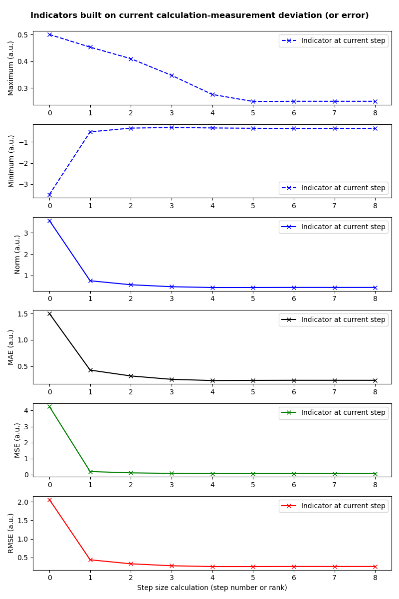
Execution of the command set gives the following results, which illustrate the series structure of the indicators, associated with the series of values of the incremental quantity “InnovationAtCurrentState” required:
Displays current state values, at each step:
  Current state: [0.0000 1.0000 2.0000]
  Current state: [0.0474 0.9053 1.0056]
  Current state: [0.0905 0.8492 0.9461]
  Current state: [0.1529 0.7984 0.9367]
  Current state: [0.2245 0.7899 0.9436]
  Current state: [0.2508 0.8005 0.9486]
  Current state: [0.2500 0.7998 0.9502]
  Current state: [0.2500 0.8000 0.9500]
  Current state: [0.2500 0.8000 0.9500]

Calculation-measurement deviation (or error) indicators
     (only the first 3 steps are displayed here)

===> Maximum error between calculations and measurements, at each step:
     [0.5000 0.4526 0.4095]
===> Minimum error between calculations and measurements, at each step:
     [-3.5000 -0.5169 -0.3384]
===> Norm of the error between calculation and measurement, at each step:
     [3.5707 0.7540 0.5670]
===> Mean absolute error (MAE) between calculations and measurements, at each step:
     [1.5000 0.4267 0.3154]
===> Mean square error (MSE) between calculations and measurements, at each step:
     [4.2500 0.1895 0.1072]
===> Root mean square error (RMSE) between calculations and measurements, at each step:
     [2.0616 0.4353 0.3274]
In graphical form, the indicators are displayed over all the steps:
- HOMARD
For more information on HOMARD, see the HOMARD module and its integrated help available from the main menu Help of the SALOME platform.
- PARAVIS
For more information on PARAVIS, see the PARAVIS module and its integrated help available from the main menu Help of the SALOME platform.
- YACS
For more information on YACS, see the YACS module and its integrated help available from the main menu Help of the SALOME platform.