FIELDS module: User guide for field manipulation

This document is a quick guide for Graphical User Interface of FIELDS module. It shows how to use this module on the basis of a few reference examples, built from use cases identified during requirement analysis stage.

Avertissement

This document is self-contained, but it is strongly advised to read the specification document (in french), at least to clarify concepts and terminology.

Avertissement

Screenshots are not up-to-date. They were extracted from SALOME 6 with data visualization achieved using VISU module. In SALOME 7, VISU module has been replaced by PARAVIS module. The look-and-feel may thus be slightly different.

General presentation of FIELDS module

The overall ergonomics of FIELDS module for field manipulation is inspired by software such as octave or scilab. It combines a graphical interface (GUI) to select and prepare data, with a textual interface (the python console, TUI) for actual work on data.

This module provides two user environments that are marked by the red and green rectangles on the screenshot below:

• The data space (dataspace), in which user defines the MED data sources (datasource), that is to say the med files from which meshes and fields are read. This data space allows for the exploration of meshes and fields provided by the different data sources.
• The workspace (workspace), in which user may drop fields selected in the source space, and then use them for example to produce new fields using the operations on fields provided by the TUI.

A typical use of field manipulation functions is:

1. Load a med file in the data space and explore its contents: meshes and fields defined on these meshes, defined for one or several time steps.
2. Select (using GUI) fields to be manipulated in workspace ; it is possible to introduce restrictions on time steps, components or groups of cells.
3. Create new fields executing algebraic operations (+,-,*,/) on fields, applying simple mathematical functions (pow, sqrt, abs), or initializing them « from scratch » on a support mesh.
4. Visually control produced fields, using PARAVIS module in SALOME, automatically controlled from user interface.
5. Save (parts of) produced fields to a med file.

Quick tour on functions available in FIELDS module

This section presents some use examples of FIELDS module like a « storyboard », illustrating the functions proposed by the module.

Avertissement

This section is under construction. Please consider that its contents and organization are still incomplete and may change until this warning is removed.

Example 1: Explore data sources

Note

This example illustrates the following functions:

• add a data source
• « Extends field series » and « Visualize » functions

At startup the field manipulation module, identified by icon , shows an empty interface:

The first step consists in adding one or several med data sources in « dataspace ». For this, user clicks on icon « Add datasource » to select a med file:

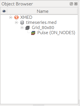
This operation adds a new entry (datasource) in data space. The contents can be explored using the data tree. The figure below (left image) shows the result of loading the file timeseries.med containing a mesh named Grid_80x80 on which a field on nodes named Pulse is defined. By default, the field composition (in terms of time steps and components) is not displayed to avoid visual congestion of data tree. User must explicitly ask for visualization using the command « Expand field timeseries » available in the field contextual menu. The result is displayed on center image. The list of field Pulse iterations can be advised.

Note

Strictly speaking, the field concept in MED model corresponds to a given iteration. A set of iterations is identified by the term field time series. If there is no ambiguity, the field name will refer to both the field itself or the time series it belongs to.

Finally, it is possible from dataspace to visualize the field general shape using a scalar map displayed in SALOME viewer. For this, user selects the time step to display then uses the command « Visualize » available in the associated contextual menu:

Note

This graphical representation aims at providing a quick visual control. Scalar maps are displayed using the PARAVIS module.

Example 2: Combine fields from different sources

Note

This example illustrates the following functions:

• function « Use in workspace »
• function « Save »

The objective is to access data contained in several med files, then to combine them in the same output file.

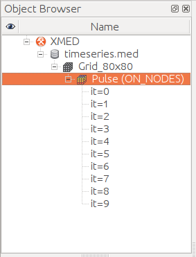
User starts by adding med data sources in dataspace. In the example below, dataspace contains two sources names parametric_01.med and smallmesh_varfiled.med. The first one contains the mesh Grid_80x80_01 on which the field StiffExp_01 is defined. The second source contains the mesh My2DMesh on which the two fields testfield1 are testfield2 are defined:

In this example, StiffExp_01 and testfield2 are combined then saved to result.med file. The procedure consists in importing the two fields in workspace, then to save the workspace. For this user selects the fields and uses the command « Use in workspace » available in the contextual menu. Both selected fields appear in the workspace tree:

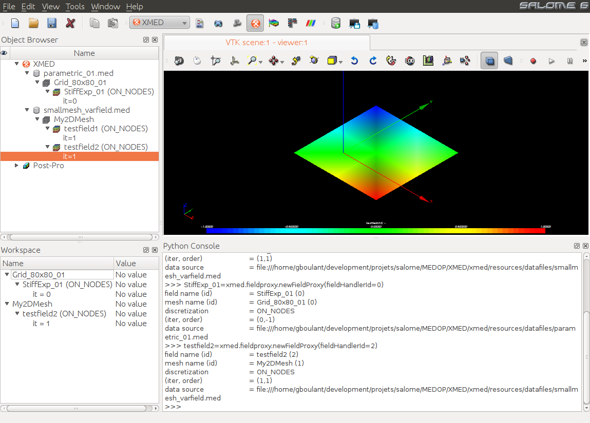
Workspace is saved using the command « Save workspace » available in the module toolbar. A dialog window lets user set the save file name:

The file result.med can then be reloaded in FIELDS module (or PARAVIS module) to check the presence of saved fields.

Example 3: Apply a formula on fields

Note

This example illustrates the following functions:

• execute mathematical operations in TUI console
• function « put » to refer to a work field in the list of persisting fields.
• function « Visualize » from TUI.

The most common usage of field manipulation module is to execute mathematical operations on fields or on their components.

Assume data sources are already defined in dataspace (in the following example a temporal series named Pulse contains 10 time steps defined on a mesh named Grid_80x80, all read from timeseries.med data source).

As previously seen, a field can be manipulated in workspace after selecting the field and applying the command « Use in workspace » from contextual menu. Here only one file is selected (two in the previous example) and the command then opens a dialog window to select data to work on and the way they will be manipulated:

Note

In the current state of development, the interface only propose to define the name of a variable representing the field in TUI. In a next version, user will have the possibility to specify the field component(s) to be used and a group of cells to introduce a geometrical restriction. Conversely it will be possible to select a complete time series to apply global operations on all time steps.

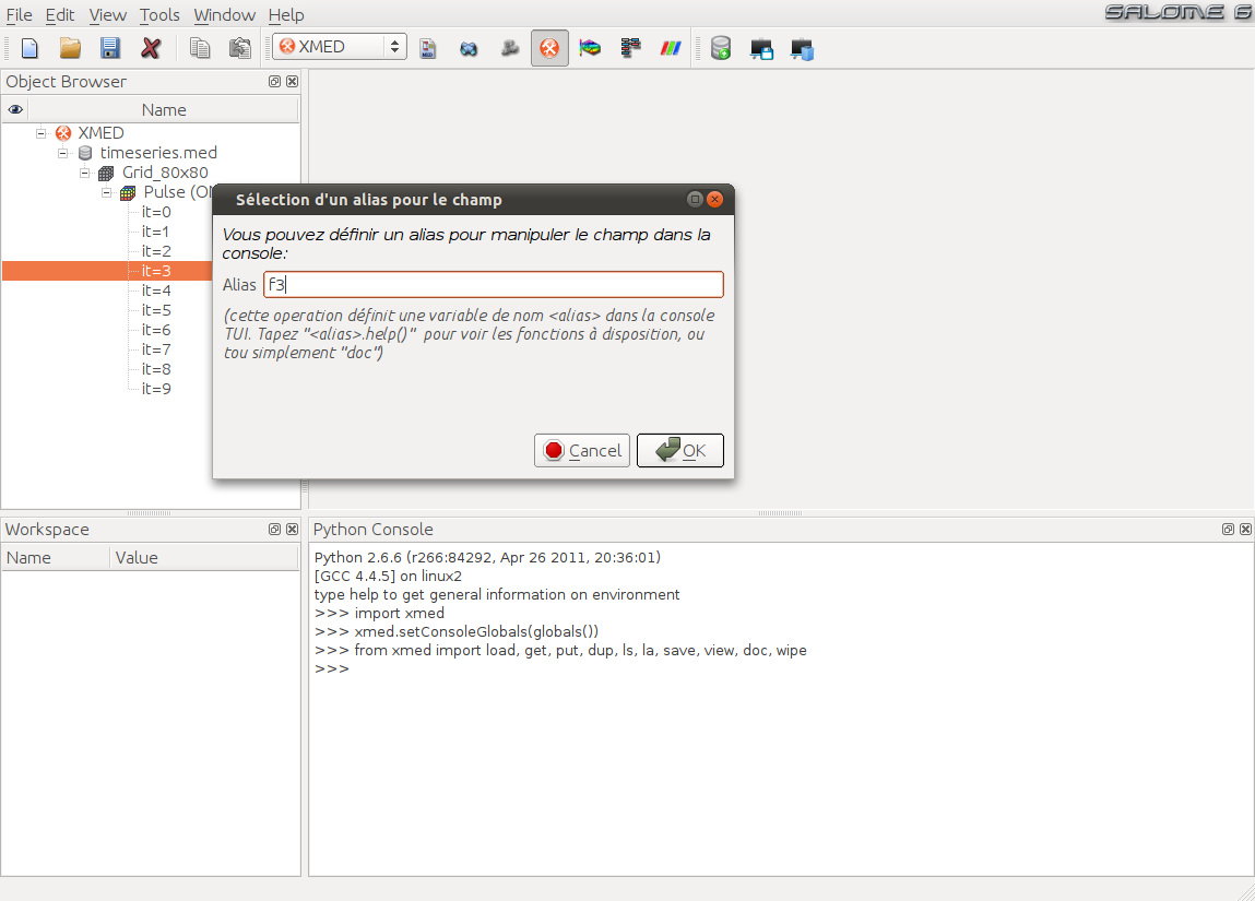
After validation, the field if put in workspace tree and a variable <alias> is automatically created in the TUI to designate the field. In this example, <alias> is f3, as set by user to recall that variable corresponds to the third time step:

Field manipulation can start. In the example below, use creates the field``r`` as the result of an affine transformation of field f3 (multiplication of field by a scale factor 2.7 then addition of offset 5.2):

>>> r=2.7*f3+5.2

Other operations can be applied, as detailed in module specifications (cf. Spécification des opérations):

>>> r=f3/1000     # the values of r are the ones of f3 reduced by a factor 1000
>>> r=1/f3        # the values of r are the inverted values of f3
>>> r=f3*f3       # the values of r are the squared values of f3
>>> r=pow(f3,2)   # same result
>>> r=abs(f3)     # absolute value of field f3
>>> ...

The two operands can be fields. If f4 is the fourth time step of field Pulse, then algebraic combinations of fields can be computed:

>>> r=f3+f4
>>> r=f3-f4
>>> r=f3/f4
>>> r=f3*f4

Scalar variables can be used if needed:

>>> r=4*f3-f4/1000
>>> ...

In these examples, the variable r corresponds to a work field containing the operation result. By default the field is nor referenced in workspace tree. If user wants to add it, for example to make it considered when saving, then the following command is used:

>>> put(r)

The function put aims at tagging the field as persisting, the to store it in the workspace tree to make it visible and selectable. Among all fields that could be created in console during the work session, all do not need to be saved. Some may only be temporary variables used in the construction of final fields. That is why only fields in workspace tree are saved when saving the workspace.

Variables defined in console have other uses. First they allow for printing information relative to the manipulated field. For this one enters the variable name then validates:

>>> f3
field name (id)         = Pulse (3)
mesh name (id)          = Grid_80x80 (0)
discretization          = ON_NODES
(iter, order)           = (3,-1)
data source             = file:///home/gboulant/development/projets/salome/MEDOP/XMED/xmed/resources/datafiles/timeseries.med

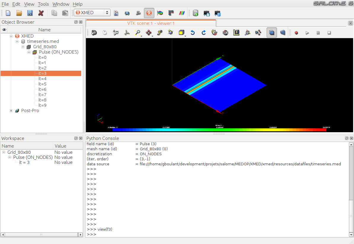
Second, variables can be used as command arguments (the list of commands available in TUI is described in section Documentation of textual interface). For example the function view displays the field scalar map in the viewer:

>>> view(f3)

Results in:

Note

It is easy to compare two time steps of a field, computing the difference f3-f4, then producing a scalar map preview using the function view:

>>> view(f3-f4)

Finally the field data can be displayed using the command``print``:

>>> print f3
Data content :
Tuple #0 : -0.6
Tuple #1 : -0.1
Tuple #2 : 0.4
Tuple #3 : -0.1
Tuple #4 : 0.4
...
Tuple #6556 : 3.5
Tuple #6557 : 3.3
Tuple #6558 : 1.5
Tuple #6559 : 0.3
Tuple #6560 : 0.2

It is important to note that operations between fields can only be applied if fields are defined on the same mesh. It corresponds to a specification of MED model that forbids operations between fields defined on meshes geometrically different. Technically it means that the conceptual objects fields must share the same conceptual object mesh.

If user do want to use fields defined on different meshes, for example to manipulate the field values at the interface of two meshes sharing a 2D geometrical area, it is necessary first to make all fields be defined on the same surface mesh using a projection operation.

Note

Such projection operations are available in the MEDCoupling library.

Another classical need is using fields defined on meshes geometrically identical, but technically different for example when they are loaded from different med files. For such a case, the MEDCoupling library proposes a function « Change support mesh » ; its use in field manipulation module is illustrated in example 4 described hereafter.

Example 4: Compare fields derived from different sources

Note

This example illustrates the following function:

• Change the underlying (support) mesh

Assume here that fields have been defined on same mesh, geometrically speaking, but saved in different med files. This occurs for example for a parametric study in which several computations are achieved with variants on some parameters of the simulated model, each computation producing a med file.

Let parametric_01.med and parametric_02.med be two med files containing the fields to compare, for example computing the difference of their values and visualizing the result.

After loading data sources user sees two meshes, this time from the technical point of view, that is to say fields are associated to different conceptual mesh objects, while geometrically identical.

However field manipulation functions do not allow operations on fields lying on different support meshes (see remark at the end of example 3).

To circumvent this issue, the module offers the function « Change underlying mesh » to replace a field mesh support by another, provided that the two meshes are geometrically identical, that is to say nodes have the same spatial coordinates.

In the proposed example, user selects the first time step of field StiffExp_01 in data source parametric_01.med, and imports it in workspace using the command « Use in workspace » . User then selects the first time step of field StiffExp_02 in data source parametric_02.med, but imports it in workspace using the command « Change underlying mesh » . The following dialog window appears to let user select the new support mesh in dataspace tree:

In this example, the support mesh Grid_80x80_01 of field StiffExp_01 to compare with is selected. After validation the workspace tree contains the field StiffExp_02 defined on mesh Grid_80x80_01:

Note

The function « Change underlying mesh » does not modify the field selected in dataspace (basic running principle of dataspace), but creates a field copy in workspace to then change support mesh. This explains the default name for field dup(<name of selected field>) (dup stands for « duplicate »).

All we have to do now is to associate a variable to this field, in order to manipulate it in TUI. This can be done using the command « Use in console » available in workspace contextual menu.

Finally, if f1 is a field from datasource parametric_01.med and f2 is a field from datasource parametric_02.med according to the above procedure, then comparison values can be achieved as explained in example 3:

>>> r=f1-f2
>>> view(r)

Note

As a general remark concerning this example, one may note:

• the geometrical equality of two meshes is constrained to a numerical error that can be technically set, but not through the module interface. This tolerance is empirically set to a standard value regarding to success of most of the use cases. The usefulness of setting this value in the interface could be later investigated.
• User must explicitly ask for changing a field support mesh, in order to compare fields coming from different data sources. This choice has been made to keep trace of modifications made on data (no modification is made without user knowing, even to improve ergonomics).

Example 5: Create a field on a spatial domain

Note

This example illustrates the following functions:

• initialize with function of spatial position
• initialize on a group of cells

The geometrical domain on which the field to create is defined is here given by cell group data. This use case is provided for producing initial load conditions of a structure, for example defining a field on a geometry surface identified by a group of cells.

Avertissement

DEVELOPMENT IN PROGRESS

Example 6: Extract a field part

Note

This example illustrates the following functions:

• extract a component (or a subset of components)
• extract a geometrical domain (values on a group of cells)
• extract one or several time steps

Avertissement

DEVELOPMENT IN PROGRESS

Here the restriction functions that allow to get some components only, have to be illustrated. The principle is creating a new field that is a restriction of input field to a list of given components (use the function __call__ of fieldproxy).

For time step extraction, we can reduce to the case of example 2 with a single data source.

Example 7: Create a field from a to[mp]ographic image

Note

This example illustrates the following function:

• Create a field without data source (neither mesh nor field), from an image file

In tomography or topography studies, measurement devices produce images that represent a physical quantity using gray levels on a given cutting plane. The following image represents for example a internal view of human body obtained by MRI:

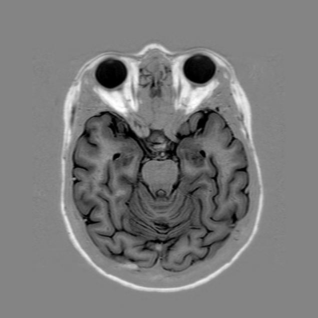
This image is a subset of pixels organized on a Cartesian grid. It can thus be represented as a scalar field whose values are defined on cells of a mesh having the same dimension as the image (number of pixels):

The field manipulation module provides a tool named image2med.py to convert a file image to a med file containing the image representation as a scalar field (only the gray level is kept):

$ <xmed_root_dir>/bin/salome/xmed/image2med.py -i myimage.png -m myfield.med

This conversion operation can be automatically achieved using the command « Add Image Source » available in GUI toolbar. This command opens the following window to let user select a file image:

The name of result med file is set by default (changing file extension to *.med) but can be modified. Finally user can ask for automatic load of this med file in data space. Fields can then be manipulated like presented in the standard use cases.

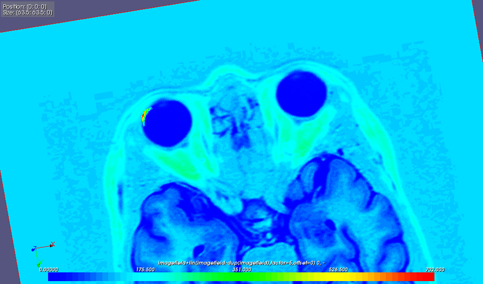
For example, the image below depicts the result of the difference between two images, added to the reference image: if i1 and i2 are the fields created from these two images, then r = i1 + 5*(i2-i1) with 5 an arbitrary factor to amplify the region of interest (above the left eye):

The example below is the result of loading a tomographic image courtesy of MAP project (Charles Toulemonde, EDF/R&D/MMC). The tomographic image:

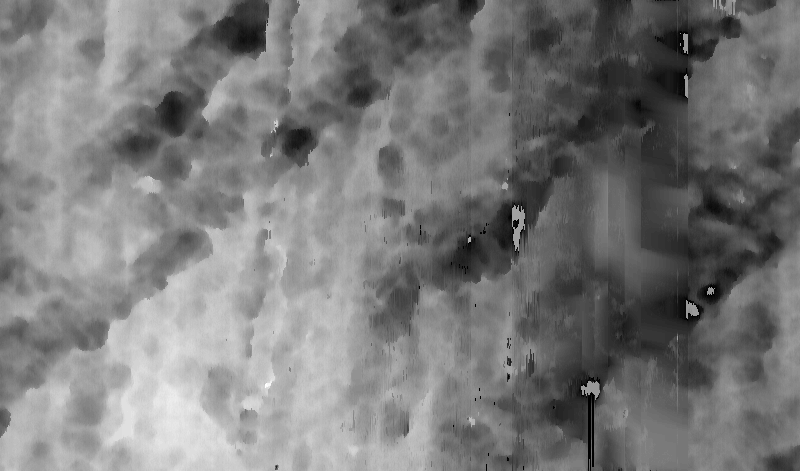
The result of loading:

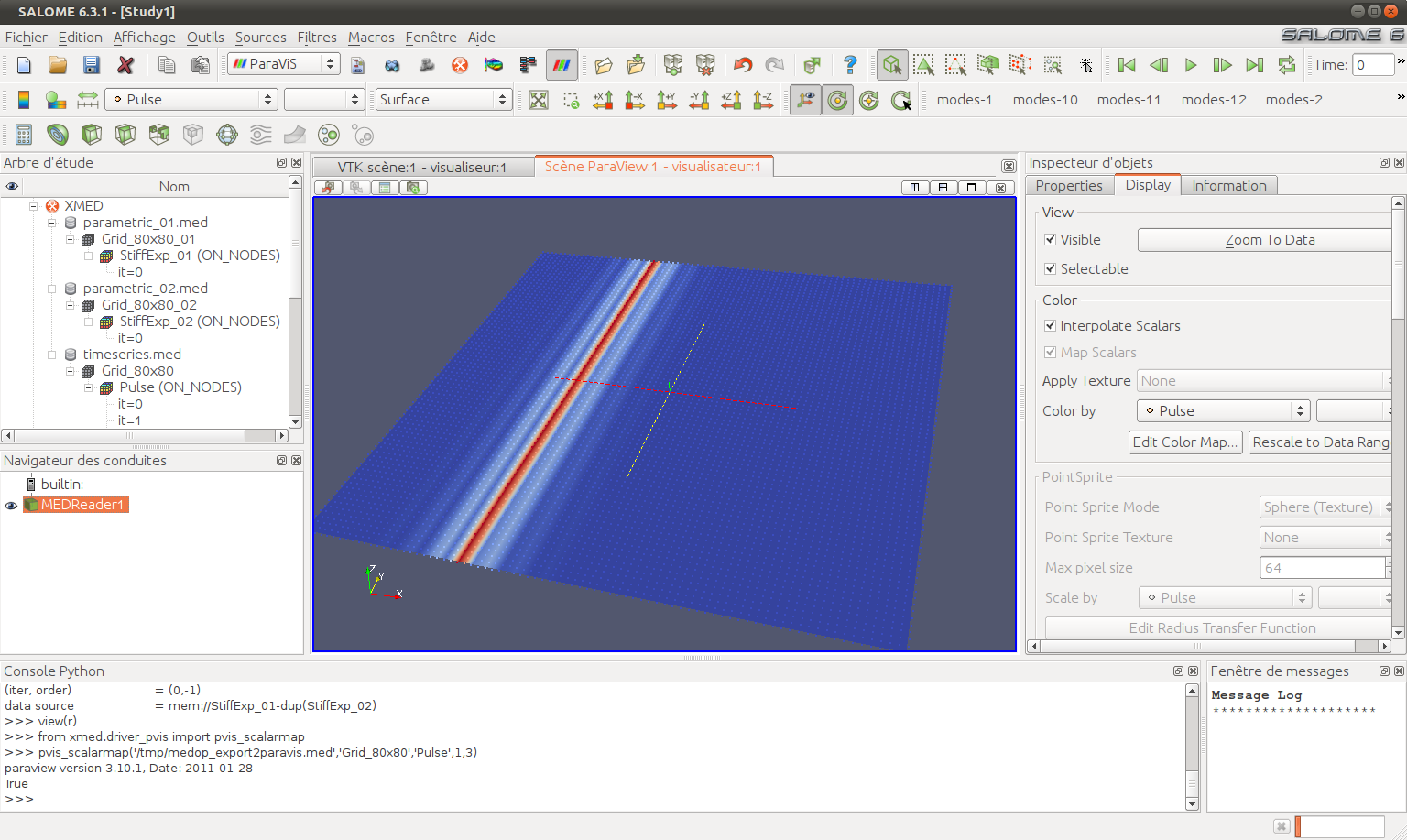
Example 8: Continue analysis in PARAVIS

Note

This example illustrates the following functio:

• Export fields to PARAVIS module

The solutions for field representation in FIELDS module aims at proposing a quick visual control.

For a detailed analysis of fields, user shall switch to PARAVIS. The field manipulation module has a function to facilitate this transition, with automatic load in PARAVIS and proposing a default visualization (scalar map).

For this user selects in workspace the fields to export, then call the export function from contextual menu:

Selected fields are grouped in a single MED entry in PARAVIS, and the first field is depicted as a scalar map:

Note

The export function is a convenience function. The same operation can be manually achieved, first saving fields to a med file then loading the created file in PARAVIS module for visualization.

Using the textual interface (TUI)

All operations driven through GUI can be done (more or less easily) using TUI. The field manipulation module can even be used exclusively in textual mode.

For this run the command:

$ <path/to/appli>/medop.sh

This command opens a command console medop>. A med file can be loaded and manipulated, for example to create fields from file data.

Whatever textual or graphical mode is used, a typical workflow in console looks like the following instructions:

>>> medcalc.LoadDataSource("/path/to/mydata.med")
>>> la
id=0    name    = testfield1
id=1    name    = testfield2
>>> f1=accessField(0)
>>> f2=accessField(1)
>>>    ls
f1      (id=0, name=testfield1)
f2      (id=1, name=testfield2)
>>> r=f1+f2
>>> ls
f1      (id=0, name=testfield1)
f2      (id=1, name=testfield2)
r       (id=2, name=testfield1+testfield2)
>>> r.update(name="toto")
>>> ls
f1      (id=0, name=testfield1)
f2      (id=1, name=testfield2)
r       (id=2, name=toto)
>>> putInWorkspace(r)
>>> saveWorkspace("result.med")

The main commands are:

• LoadDataSource: load a med file in data base (useful in pure textual mode):

  >>> LoadDataSource("/path/to/datafile.med")
  

• LoadImageAsDataSource: load an image as a med file

• la: show the list of all fields loaded in data base (« list all »)

• accessField: set a field in workspace from its identifier (useful in pure textual mode ; this operation can be done in GUI selecting a field from data space).:

  >>> f=accessField(fieldId)
  

• ls: show the list of fields available in workspace (« list »)

• putInWorkspace: put a reference to a field in management space:

  >>> putInWorkspace(f)
  

• saveWorkspace: save to a med a file all fields referenced in management space:

  >>> saveWorkspace("/path/to/resultfile.med")
  

Note

• the LoadDataSource command only loads metadata describing meshes and fields (names, discretization types, list of time steps). Meshes and physical quantities on fields are loaded later (and automatically) as soon as an operation needs them. In all cases med data (mete-information and values) are physically stored in data base environment.
• the accessField command defines a field handler in workspace, i.e. a variable that links to the physical field hosted in data base. Physical data never transit between environments but remain centralized in data base.

The following TUI commands need to work in graphical environment:

• medcalc.MakeDeflectionShape
• medcalc.MakeIsoSurface
• medcalc.MakePointSprite
• medcalc.MakeScalarMap
• medcalc.MakeSlices
• medcalc.MakeVectorField