14.12. Checking algorithm “ReducedModelingTest”
This algorithm is reserved for use in the textual user interface (TUI), and therefore not in graphical user interface (GUI).
14.12.1. Description
This algorithm provides a simple analysis of the characteristics of the state collection from the point of view of reduction. It aims to diagnose the complexity of the information present in the available state collection, and the possibility to represent this state information in a space smaller than the entire state collection. Technically, based on a classical SVD (Singular Value Decomposition) and in the same way as a PCA (Principal Component Analysis), it evaluates how information decreases with the number of singular values, either as values or, from a statistical point of view, as remaining variance.
Once the analysis is complete, a summary is displayed and, on request, a graphical representation of the same information is produced.
14.12.2. Some noteworthy properties of the implemented methods
To complete the description, we summarize here a few notable properties of the algorithm methods or of their implementations. These properties may have an influence on how it is used or on its computational performance. For further information, please refer to the more comprehensive references given at the end of this algorithm description.
The methods proposed by this algorithm do not require derivation of the objective function or of one of the operators, thus avoiding this additional calculation time when derivatives are calculated numerically by multiple evaluations.
14.12.3. Optional and required commands
The general required commands, available in the editing user graphical or textual interface, are the following:
- EnsembleOfSnapshots
List of vectors or matrix. This key contains an ordered collection of physical state vectors
 , called “snapshots” in reduced
basis terminology. At each step index, there is 1 state per column if this
list is in matrix form, or 1 state per element if it’s actually a list.
Caution: the numbering of the support or points, on which or to which a state
value is given in each vector, is implicitly that of the natural order of
numbering of the state vector, from 0 to the “size minus 1” of this vector.
, called “snapshots” in reduced
basis terminology. At each step index, there is 1 state per column if this
list is in matrix form, or 1 state per element if it’s actually a list.
Caution: the numbering of the support or points, on which or to which a state
value is given in each vector, is implicitly that of the natural order of
numbering of the state vector, from 0 to the “size minus 1” of this vector.Example :
{"EnsembleOfSnapshots":[y1, y2, y3...]}
- ExcludeLocations
List of integers or names. This key specifies the list of points in the state vector excluded from the optimal search. The default value is an empty list. The list can contain either indices of points (in the implicit internal order of a state vector) or names of points (which must exist in the list of position names indicated by the keyword “NameOfLocations” in order to be excluded). By default, if the elements of the list are strings that can be assimilated to indices, then these strings are indeed considered as indices and not names.
Important notice: the numbering of these excluded points must be identical to that adopted, implicitly and imperatively, by the variables constituting a state considered arbitrarily in one-dimensional form.
Example :
{"ExcludeLocations":[3, 125, 286]}or{"ExcludeLocations":["Point3", "XgTaC"]}
- MaximumNumberOfLocations
Integer value. This key specifies the maximum possible number of positions found in the optimal search. The default value is 1. The optimal search may eventually find less positions than required by this key, as for example in the case where the residual associated to the approximation is lower than the criterion and leads to the early termination of the optimal search. It is recommended to adapt this parameter to the needs on real problems.
Example :
{"MaximumNumberOfLocations":5}
- MaximumNumberOfModes
Integer value. This key indicates the maximum possible number of decomposition modes to be included in the reduction analysis. The default value is 1.e6, which is very similar to no limit on this number of modes, and it is recommended to adapt it to the needs of real problems.
Example :
{"MaximumNumberOfModes":5}
- NameOfLocations
List of names. This key indicates an explicit list of variable names or positions, positioned as in a state vector considered arbitrarily in one-dimensional form. The default value is an empty list. To be used, this list must have the same length as that of a physical state.
Important notice: the order of the names is, implicitly and imperatively, the same as that of the variables constituting a state considered arbitrarily in one-dimensional form.
Example :
{"NameOfLocations":["Point3", "Location42", "Position125", "XgTaC"]}
- NumberOfPrintedDigits
Integer value. This key indicates the number of digits of precision for floating point printed output. The default is 5, with a minimum of 0.
Example:
{"NumberOfPrintedDigits":5}
- PlotAndSave
Boolean value. The variable leads to the display of results in graphical form and the saving in a file of an associated figure. The default is “False”, the choices are “True” or “False”.
Example :
{"PlotAndSave":False}
- SampleAsExplicitHyperCube
List of list of real values. This key describes the calculations points as an hyper-cube, from a given list of explicit sampling of each variable as a list. That is then a list of lists, each of them being potentially of different size. By nature, the points are included in the domain defined by the bounds of the explicit lists for each variable.
Example :
{"SampleAsExplicitHyperCube":[[0.,0.25,0.5,0.75,1.], [-2,2,1]]}for a state space of dimension 2.
- SampleAsIndependentRandomVariables
List of triplets [Name, Parameters, Number]. This key describes the calculations points as an hyper-cube, for which the points on each axis come from a independent random sampling of the axis variable, under the specification of the distribution, its parameters and the number of points in the sample, as a list [Name, Parameters, Number] for each axis. Unlike sampling described by the keyword “SampleAsIndependentRandomVectors”, points are explicitly distributed over a regular hypercube. The possible distribution names are ‘normal’ of parameters (mean,std), ‘lognormal’ of parameters (mean,sigma), ‘uniform’ of parameters (low,high), or ‘weibull’ of parameter (shape). That is then a list of the same size than the one of the state. By nature, the points are included in the unbounded or bounded domain, depending on the characteristics of the distributions chosen for each variable.
Example :
{"SampleAsIndependentRandomVariables":[['normal',[0.,1.],3], ['uniform',[-2,2],4]]}for a state space of dimension 2.
- SampleAsIndependentRandomVectors
List of pairs [Name, Parameters], plus [Dimension, Number]. This key describes the calculation points in the form of particular distributions defined for each dimension, resulting in random vectors whose individual components follow the required distribution. Unlike the sampling described by the keyword “SampleAsIndependentRandomVariables”, the points are not distributed over a regular hypercube. The distribution on each axis variable is specified by its name and parameters, in the form of a list [Name, Parameters] for each axis. This list of pairs, whose number is identical to the size of the state space, is completed by a pair of integers [Dimension, Number] containing the dimension of the state space and the desired number of sampling points. Possible distribution names are ‘normal’ with parameters (mean,std), ‘lognormal’ with parameters (mean,sigma), ‘uniform’ with parameters (low,high), ‘loguniform’ with parameters (low,high), or ‘weibull’ with parameters (shape). By their very nature, points are included in the unbounded or bounded domain, depending on the characteristics of the distributions chosen for each variable. Distributions can be different for each axis.
Example :
{"SampleAsIndependentRandomVectors":[['normal',[0.,1.]], ['uniform',[-2,2]]]}for a state space of dimension 2.
- SampleAsMinMaxLatinHyperCube
List of real valued pairs [Min, Max], plus [Dimension, Number]. This key describes the bounded domain in which the calculations points will be placed, from a [Min, Max] pair for each state component. The lower bounds are included. This list of pairs, identical in number to the size of the state space, is augmented by a pair of integers [Dimension, Number] containing the dimension of the state space and the desired number of sample points. Sampling is then automatically constructed using the Latin hypercube method (LHS). By nature, the points are included in the domain defined by the explicit bounds.
Example :
{"SampleAsMinMaxLatinHyperCube":[[0.,1.],[-1,3]]+[[2,11]]}for a state space of dimension 2 and for 11 sampling points.
- SampleAsMinMaxSobolSequence
List of real valued pairs [Min, Max], plus [Dimension, Number]. This key describes the bounded domain in which the calculations points will be placed, from a [Min, Max] pair for each state component. The lower bounds are included. This list of pairs, identical in number to the size of the state space, is augmented by a pair of integers [Dimension, Number] containing the dimension of the state space and the minimum desired number of sample points (by construction, the number of points generated in the Sobol sequence will be the power of 2 immediately above this minimum number). Sampling is then automatically constructed using the Sobol sequence method. By nature, the points are included in the domain defined by the explicit bounds.
Remark: it is required to have Scipy version 1.7.0 or higher to use this sampling option.
Example :
{"SampleAsMinMaxSobolSequence":[[0.,1.],[-1,3]]+[[2,11]]}for a state space of dimension 2 and 11 sampling points (there will be 16 points in practice).
- SampleAsMinMaxStepHyperCube
List of triplets of real values [Min, Max, Step]. This key describes the calculations points as an hyper-cube, from a given list of implicit sampling of each variable by a triplet [Min, Max, Step]. That is then a list of the same size than the one of the state. The bounds are included. By nature, the points are included in the domain defined by the explicit bounds.
Example :
{"SampleAsMinMaxStepHyperCube":[[0.,1.,0.25],[-1,3,1]]}for a state space of dimension 2.
- SampleAsnUplet
List of states. This key describes the calculations points as a list of n-uplets, each n-uplet being a state. By nature, points are included in the bounded domain defined as the convex envelope of explicitly designated points.
Example :
{"SampleAsnUplet":[[0,1,2,3],[4,3,2,1],[-2,3,-4,5]]}for 3 points in a state space of dimension 4.
- SetDebug
Boolean value. This variable leads to the activation, or not, of the debug mode during the function or operator evaluation. The default is “False”, the choices are “True” or “False”.
Example:
{"SetDebug":False}
- SetSeed
Integer value. This key allow to give an integer in order to fix the seed of the random generator used in the algorithm. By default, the seed is left uninitialized, and so use the default initialization from the computer, which then change at each study. To ensure the reproducibility of results involving random samples, it is strongly advised to initialize the seed. A simple convenient value is for example 123456789. It is recommended to put an integer with more than 6 or 7 digits to properly initialize the random generator.
Example:
{"SetSeed":123456789}
- ShowElementarySummary
Boolean value. This variable leads to the activation, or not, of the calculation and display of a summary at each elementary evaluation of the test. The default value is “True”, the choices are “True” or “False”.
Example :
{"ShowElementarySummary":False}- StoreSupplementaryCalculations
List of names. This list indicates the names of the supplementary variables, that can be available during or at the end of the algorithm, if they are initially required by the user. Their availability involves, potentially, costly calculations or memory consumptions. The default is then a void list, none of these variables being calculated and stored by default (excepted the unconditional variables). The possible names are in the following list (the detailed description of each named variable is given in the following part of this specific algorithmic documentation, in the sub-section “Information and variables available at the end of the algorithm”): [ “EnsembleOfSimulations”, “EnsembleOfStates”, “Residus”, “SingularValues”, ].
Example :
{"StoreSupplementaryCalculations":["CurrentState", "Residu"]}
14.12.4. Information and variables available at the end of the algorithm
At the output, after executing the algorithm, there are information and
variables originating from the calculation. The description of
Variables and information available at the output show the way to obtain them by the method
named get, of the variable “ADD” of the post-processing in graphical
interface, or of the case in textual interface. The input variables, available
to the user at the output in order to facilitate the writing of post-processing
procedures, are described in an Inventory of potentially available information at the output.
Permanent outputs (non conditional)
The unconditional outputs of the algorithm are the following:
None
Set of on-demand outputs (conditional or not)
The whole set of algorithm outputs (conditional or not), sorted by alphabetical order, is the following:
- EnsembleOfSimulations
List of vectors or matrix. This key contains an ordered collection of physical state vectors or simulated state vectors
that may
be observed. These are  operator outputs, i.e. simulated
observation states (called “snapshots” in reduced-base terminology). At
each step index, there is 1 state per column if this list is in matrix form,
or 1 state per element if it’s actually a list. Caution: the numbering of the
support or points, on which or to which a state value is given in each
vector, is implicitly that of the natural order of numbering of the state
vector, from 0 to the “size minus 1” of this vector.
operator outputs, i.e. simulated
observation states (called “snapshots” in reduced-base terminology). At
each step index, there is 1 state per column if this list is in matrix form,
or 1 state per element if it’s actually a list. Caution: the numbering of the
support or points, on which or to which a state value is given in each
vector, is implicitly that of the natural order of numbering of the state
vector, from 0 to the “size minus 1” of this vector.Example :
{"EnsembleOfSimulations":[y1, y2, y3...]}
- EnsembleOfStates
List of vectors or matrix. Each element is an ordered collection of physical or parameter state vectors
 . These are
operator entries, i.e. current states before observation. At each step
index, there is 1 state per column if this list is in matrix form, or 1 state
per element if it’s actually a list. Caution: the numbering of the support or
points, on which or to which a state value is given in each vector, is
implicitly that of the natural order of numbering of the state vector, from 0
to the “size minus 1” of this vector.
. These are
operator entries, i.e. current states before observation. At each step
index, there is 1 state per column if this list is in matrix form, or 1 state
per element if it’s actually a list. Caution: the numbering of the support or
points, on which or to which a state value is given in each vector, is
implicitly that of the natural order of numbering of the state vector, from 0
to the “size minus 1” of this vector.Example :
{"EnsembleOfStates":[x1, x2, x3...]}
- Residus
List of real value series. Each element is a series, containing the values of the particular residue checked during the running of the algorithm.
Example :
rs = ADD.get("Residus")[-1]
- SingularValues
List of real value series. Each element is a series, containing the singular values obtained through a SVD decomposition of a collection of full state vectors. The number of singular values is not limited by the requested size of the reduced basis.
Example :
sv = ADD.get("SingularValues")[-1]
14.12.5. Python (TUI) use examples
Here is one or more very simple examples of the proposed algorithm and its parameters, written in [DocR] Textual User Interface for ADAO (TUI/API). Moreover, when it is possible, the information given as input also allows to define an equivalent case in [DocR] Graphical User Interface for ADAO (GUI/EFICAS).
14.12.5.1. First example
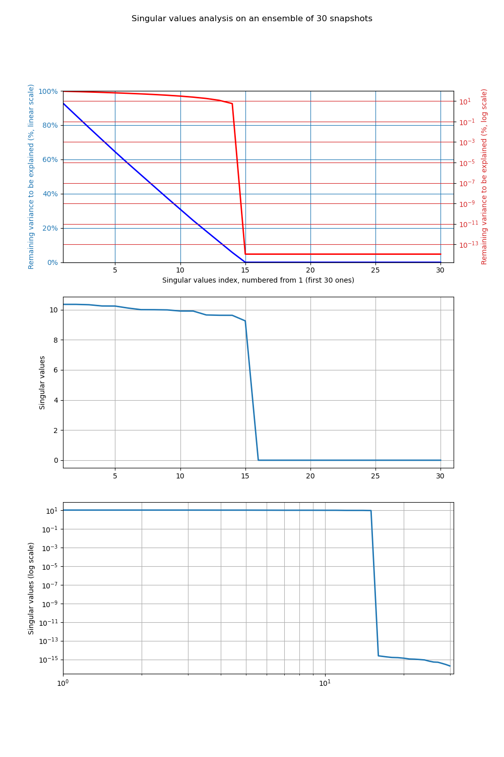
This example describes the reducibility characteristics of the set of states (“snapshots”) under study. The set considered is first composed of 15 sine calculations on a sequence of integers (so the space generated by the snapshots is linearly non-decomposable) and these 15 snapshots are then duplicated once to obtain a reduced space of size exactly 15 (since the last 15 are identical to the first 15). All the variance is thus explained by the first 15 modes, numbered from 0 to 14, and the following singular values are close to numerical zero.
# -*- coding: utf-8 -*-
#
import numpy
from adao import adaoBuilder
numpy.random.seed(123456789)
#
dimension = 100
nbsnapshots = 15
Ensemble = numpy.empty((dimension,2*nbsnapshots))
for i in range(nbsnapshots):
    Ensemble[:,i] = numpy.sin((i+1)*numpy.arange(dimension))
Ensemble[:,nbsnapshots:2*nbsnapshots] = Ensemble[:,:nbsnapshots]
#
case = adaoBuilder.New()
case.setAlgorithmParameters(
    Algorithm = "ReducedModelingTest",
    Parameters = {
        "EnsembleOfSnapshots":Ensemble,
        "StoreSupplementaryCalculations":["Residus","SingularValues"],
        "PlotAndSave":True,
        "ResultFile":"simple_ReducedModelingTest1.png",
        }
    )
case.execute()
The execution result is the following:
     REDUCEDMODELINGTEST
     ===================

     This test allows to analyze the characteristics of the collection of
     states from a reduction point of view. Using an SVD, it measures how
     the information decreases with the number of singular values, either
     as values or, with a statistical point of view, as remaining variance.

===> Information before launching:
     -----------------------------

     Characteristics of input data:
       State dimension................: 100
       Number of snapshots to test....: 30

===> Summary of the 5 first singular values:
     ---------------------------------------

     Singular values σ:
       σ[1] = 1.03513e+01
       σ[2] = 1.03509e+01
       σ[3] = 1.03258e+01
       σ[4] = 1.02436e+01
       σ[5] = 1.02386e+01

     Singular values σ divided by the first one σ[1]:
       σ[1] / σ[1] = 1.00000e+00
       σ[2] / σ[1] = 9.99962e-01
       σ[3] / σ[1] = 9.97533e-01
       σ[4] / σ[1] = 9.89589e-01
       σ[5] / σ[1] = 9.89104e-01

===> Ordered singular values and remaining variance:
     -----------------------------------------------

     -------------------------------------------------------------------------
        i  | Singular value σ |        σ[i]/σ[1] | Variance: part, remaining
     -------------------------------------------------------------------------
       00  |      1.03513e+01 |      1.00000e+00 |            7% ,    92.8%
       01  |      1.03509e+01 |      9.99962e-01 |            7% ,    85.6%
       02  |      1.03258e+01 |      9.97533e-01 |            7% ,    78.5%
       03  |      1.02436e+01 |      9.89589e-01 |            7% ,    71.5%
       04  |      1.02386e+01 |      9.89104e-01 |            7% ,    64.4%
       05  |      1.01050e+01 |      9.76200e-01 |            6% ,    57.6%
       06  |      9.99948e+00 |      9.66009e-01 |            6% ,    50.9%
       07  |      9.99643e+00 |      9.65714e-01 |            6% ,    44.2%
       08  |      9.98375e+00 |      9.64489e-01 |            6% ,    37.5%
       09  |      9.90828e+00 |      9.57198e-01 |            6% ,    31.0%
       10  |      9.90691e+00 |      9.57066e-01 |            6% ,    24.4%
       11  |      9.64803e+00 |      9.32056e-01 |            6% ,    18.1%
       12  |      9.62587e+00 |      9.29916e-01 |            6% ,    11.9%
       13  |      9.62344e+00 |      9.29681e-01 |            6% ,     5.7%
       14  |      9.25446e+00 |      8.94035e-01 |            5% ,     0.0%
       15  |      2.41400e-15 |      2.33206e-16 |            0% ,     0.0%
       16  |      1.94612e-15 |      1.88006e-16 |            0% ,     0.0%
       17  |      1.61527e-15 |      1.56044e-16 |            0% ,     0.0%
       18  |      1.54864e-15 |      1.49608e-16 |            0% ,     0.0%
       19  |      1.35243e-15 |      1.30653e-16 |            0% ,     0.0%
       20  |      1.11119e-15 |      1.07347e-16 |            0% ,     0.0%
       21  |      1.05852e-15 |      1.02260e-16 |            0% ,     0.0%
       22  |      9.68764e-16 |      9.35883e-17 |            0% ,     0.0%
       23  |      8.82878e-16 |      8.52912e-17 |            0% ,     0.0%
       24  |      6.53296e-16 |      6.31122e-17 |            0% ,     0.0%
       25  |      5.21872e-16 |      5.04159e-17 |            0% ,     0.0%
       26  |      4.98146e-16 |      4.81238e-17 |            0% ,     0.0%
       27  |      3.74898e-16 |      3.62173e-17 |            0% ,     0.0%
       28  |      2.79953e-16 |      2.70452e-17 |            0% ,     0.0%
       29  |      1.99083e-16 |      1.92326e-17 |            0% ,     0.0%
     -------------------------------------------------------------------------

===> Summary of variance cut-off:
     ----------------------------
     Representing more than 90%    of variance requires at least 14 mode(s).
     Representing more than 99%    of variance requires at least 15 mode(s).
     Representing more than 99.9%  of variance requires at least 15 mode(s).
     Representing more than 99.99% of variance requires at least 15 mode(s).

     Plot and save results in a file named "simple_ReducedModelingTest1.png"

     ---------------------------------------------------------------------------

     End of the "REDUCEDMODELINGTEST" verification

     ---------------------------------------------------------------------------
The figures illustrating the result of its execution are as follows:
14.12.6. See also
References to other sections: