15.3. Task algorithm “MeasurementsOptimalPositioningTask”¶

This algorithm is reserved for use in the textual user interface (TUI), and therefore not in graphical user interface (GUI).

15.3.1. Description¶

This algorithm provides optimal positioning of measurements of an $\mathbf{y}$ physical field, in order to get the best possible interpolation. These optimal measurement positions are determined in an iterative greedy way, from a pre-existing set of state vectors $\mathbf{y}$ (usually called “snapshots*” in reduced basis methodology) or obtained by simulating the physical field(s) of interest during the course of the algorithm. Each of these state vectors is usually (but not necessarily) the result $\mathbf{y}$ of a simulation using the operator $H$ that returns the complete field(s) for a given set of parameters $\mathbf{x}$ , or of an explicit observation of the complete field(s) $\mathbf{y}$ .

To determine the optimum positioning of measurements, an Empirical Interpolation Method (EIM [Barrault04]) or Discrete Empirical Interpolation Method (DEIM [Chaturantabut10]) is used, which establishes a reduced model of type Reduced Order Model (ROM), with (variant “lcEIM” or “lcDEIM”) or without (variant “EIM” or “DEIM”) positioning constraints. Technically, these methods build an approximation of the $\mathbf{y}$ state in a reduced-dimensional space, using a set of special interpolation points to optimally represent the global behavior of the $\mathbf{y}$ field. For performance, we recommend using the variant “lcEIM” or “EIM” when the dimension of the full fields space is large.

There are two ways to use this algorithm:

In its simplest use, if the set of physical state $\mathbf{y}$ vectors is pre-existing, it is only necessary to provide it as an ordered collection by the algorithm option “EnsembleOfSnapshots”. This is the default situation, for example, if the set of states has been generated by an Task algorithm “EnsembleOfSimulationGenerationTask”.
If the set of physical state $\mathbf{y}$ vectors is to be obtained by explicit simulations during the course of the algorithm, then one must provide both the simulation operator of the complete field, here identified with the observation operator $H$ of the complete field, and the design of experiment of the space of parametric states $\mathbf{x}$ .

If the design of experiments is supplied, the sampling of the states $\mathbf{x}$ can be given as in the Task algorithm “EnsembleOfSimulationGenerationTask”, explicitly or under form of hypercubes, explicit or sampled according to classic distributions, or using Latin hypercube sampling (LHS) or Sobol sequences. The computations are optimized according to the computer resources available and the options requested by the user. You can refer to the Requirements for describing a state sampling for an illustration of sampling. Beware of the size of the hypercube (and then to the number of computations) that can be reached, it can grow quickly to be quite large. The memory required is then the product of the size of an individual $\mathbf{y}$ state and the size of the hypercube.

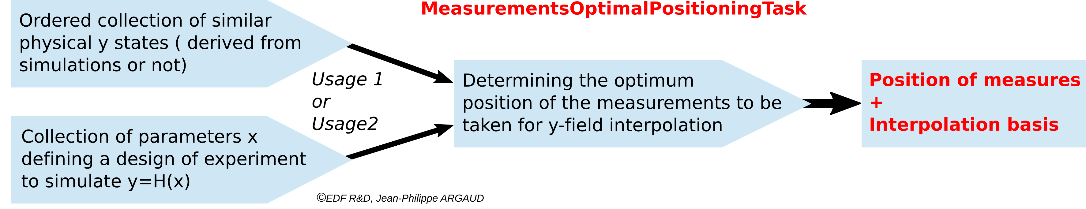
General scheme for using the algorithm

It is possible to exclude a priori potential positions for measurement positioning, using the analysis variant “lcEIM” or “lcDEIM” for a constrained positioning search.

15.3.2. Some noteworthy properties of the implemented methods¶

To complete the description, we summarize here a few notable properties of the algorithm methods or of their implementations. These properties may have an influence on how it is used or on its computational performance. For further information, please refer to the more comprehensive references given at the end of this algorithm description.

The methods proposed by this algorithm do not require derivation of the objective function or of one of the operators, thus avoiding this additional calculation time when derivatives are calculated numerically by multiple evaluations.

The methods proposed by this algorithm have internal parallelism, and can therefore take advantage of computational distribution resources. The potential interaction, between the parallelism of the numerical derivation, and the parallelism that may be present in the observation or evolution operators embedding user codes, must therefore be carefully tuned.

15.3.3. Optional and required commands¶

The general required commands, available in the editing user graphical or textual interface, are the following:

None

The general optional commands, available in the editing user graphical or textual interface, are indicated in List of commands and keywords for a dedicated task or study oriented case. Moreover, the parameters of the command “AlgorithmParameters” allow to choose the specific options, described hereafter, of the algorithm. See Description of options of an algorithm by “AlgorithmParameters” for the good use of this command.

The options are the following:

EnsembleOfSnapshots

List of vectors or matrix. This key contains an ordered collection of physical state vectors $\mathbf{y}$ , called “snapshots” in reduced basis terminology. At each step index, there is 1 state per column if this list is in matrix form, or 1 state per element if it’s actually a list. Caution: the numbering of the support or points, on which or to which a state value is given in each vector, is implicitly that of the natural order of numbering of the state vector, from 0 to the “size minus 1” of this vector.

Example : {"EnsembleOfSnapshots":[y1, y2, y3...]}

ExcludeLocations

List of integers or names. This key specifies the list of points in the state vector excluded from the optimal search. The default value is an empty list. The list can contain either indices of points (in the implicit internal order of a state vector) or names of points (which must exist in the list of position names indicated by the keyword “NameOfLocations” in order to be excluded). By default, if the elements of the list are strings that can be assimilated to indices, then these strings are indeed considered as indices and not names.

Important notice: the numbering of these excluded points must be identical to that adopted, implicitly and imperatively, by the variables constituting a state considered arbitrarily in one-dimensional form.

Example : {"ExcludeLocations":[3, 125, 286]} or {"ExcludeLocations":["Point3", "XgTaC"]}

ErrorNorm

Predefined name. This key indicates the norm used for the residue that controls the optimal search. The default is the “L2” norm. The possible criteria are in the following list: [“L2”, “Linf”].

Example : {"ErrorNorm":"L2"}

ErrorNormTolerance

Real value. This key specifies the value at which the residual associated with the approximation is acceptable, which leads to stop the optimal search. The default value is 1.e-7 (which is usually equivalent to almost no stopping criterion because the approximation is less precise), and it is recommended to adapt it to the needs for real problems. A usual value, recommended to stop the search on residual criterion, is 1.e-2.

Example : {"ErrorNormTolerance":1.e-7}

MaximumNumberOfLocations

Integer value. This key specifies the maximum possible number of positions found in the optimal search. The default value is 1. The optimal search may eventually find less positions than required by this key, as for example in the case where the residual associated to the approximation is lower than the criterion and leads to the early termination of the optimal search. It is recommended to adapt this parameter to the needs on real problems.

Example : {"MaximumNumberOfLocations":5}

NameOfLocations

List of names. This key indicates an explicit list of variable names or positions, positioned as in a state vector considered arbitrarily in one-dimensional form. The default value is an empty list. To be used, this list must have the same length as that of a physical state.

Important notice: the order of the names is, implicitly and imperatively, the same as that of the variables constituting a state considered arbitrarily in one-dimensional form.

Example : {"NameOfLocations":["Point3", "Location42", "Position125", "XgTaC"]}

ReduceMemoryUse

Boolean value. The variable leads to the activation, or not, of the memory footprint reduction mode at runtime, at the cost of a potential increase in calculation time. Results may differ above a certain precision (1.e-12 to 1.e-14), usually close to machine precision (1.e-16). The default is “False”, the choices are “True” or “False”.

Example: {"ReduceMemoryUse":False}

SampleAsExplicitHyperCube

List of list of real values. This key describes the calculations points as an hyper-cube, from a given list of explicit sampling of each variable as a list. That is then a list of lists, each of them being potentially of different size. By nature, the points are included in the domain defined by the bounds of the explicit lists for each variable.

Example : {"SampleAsExplicitHyperCube":[[0.,0.25,0.5,0.75,1.], [-2,2,1]]} for a state space of dimension 2.

SampleAsIndependentRandomVariables

List of triplets [Name, Parameters, Number]. This key describes the calculations points as an hyper-cube, for which the points on each axis come from a independent random sampling of the axis variable, under the specification of the distribution, its parameters and the number of points in the sample, as a list [Name, Parameters, Number] for each axis. Unlike sampling described by the keyword “SampleAsIndependentRandomVectors”, points are explicitly distributed over a regular hypercube. The possible distribution names are ‘normal’ of parameters (mean,std), ‘lognormal’ of parameters (mean,sigma), ‘uniform’ of parameters (low,high), or ‘weibull’ of parameter (shape). That is then a list of the same size than the one of the state. By nature, the points are included in the unbounded or bounded domain, depending on the characteristics of the distributions chosen for each variable.

Example : {"SampleAsIndependentRandomVariables":[['normal',[0.,1.],3], ['uniform',[-2,2],4]]} for a state space of dimension 2.

SampleAsIndependentRandomVectors

List of pairs [Name, Parameters], plus [Dimension, Number]. This key describes the calculation points in the form of particular distributions defined for each dimension, resulting in random vectors whose individual components follow the required distribution. Unlike the sampling described by the keyword “SampleAsIndependentRandomVariables”, the points are not distributed over a regular hypercube. The distribution on each axis variable is specified by its name and parameters, in the form of a list [Name, Parameters] for each axis. This list of pairs, whose number is identical to the size of the state space, is completed by a pair of integers [Dimension, Number] containing the dimension of the state space and the desired number of sampling points. Possible distribution names are ‘normal’ with parameters (mean,std), ‘lognormal’ with parameters (mean,sigma), ‘uniform’ with parameters (low,high), ‘loguniform’ with parameters (low,high), or ‘weibull’ with parameters (shape). By their very nature, points are included in the unbounded or bounded domain, depending on the characteristics of the distributions chosen for each variable. Distributions can be different for each axis.

Example : {"SampleAsIndependentRandomVectors":[['normal',[0.,1.]], ['uniform',[-2,2]]]} for a state space of dimension 2.

SampleAsMinMaxLatinHyperCube

List of real valued pairs [Min, Max], plus [Dimension, Number]. This key describes the bounded domain in which the calculations points will be placed, from a [Min, Max] pair for each state component. The lower bounds are included. This list of pairs, identical in number to the size of the state space, is augmented by a pair of integers [Dimension, Number] containing the dimension of the state space and the desired number of sample points. Sampling is then automatically constructed using the Latin hypercube method (LHS). By nature, the points are included in the domain defined by the explicit bounds.

Example : {"SampleAsMinMaxLatinHyperCube":[[0.,1.],[-1,3]]+[[2,11]]} for a state space of dimension 2 and for 11 sampling points.

SampleAsMinMaxSobolSequence

List of real valued pairs [Min, Max], plus [Dimension, Number]. This key describes the bounded domain in which the calculations points will be placed, from a [Min, Max] pair for each state component. The lower bounds are included. This list of pairs, identical in number to the size of the state space, is augmented by a pair of integers [Dimension, Number] containing the dimension of the state space and the minimum desired number of sample points (by construction, the number of points generated in the Sobol sequence will be the power of 2 immediately above this minimum number). Sampling is then automatically constructed using the Sobol sequence method. By nature, the points are included in the domain defined by the explicit bounds.

Remark: it is required to have Scipy version 1.7.0 or higher to use this sampling option.

Example : {"SampleAsMinMaxSobolSequence":[[0.,1.],[-1,3]]+[[2,11]]} for a state space of dimension 2 and 11 sampling points (there will be 16 points in practice).

SampleAsMinMaxStepHyperCube

List of triplets of real values [Min, Max, Step]. This key describes the calculations points as an hyper-cube, from a given list of implicit sampling of each variable by a triplet [Min, Max, Step]. That is then a list of the same size than the one of the state. The bounds are included. By nature, the points are included in the domain defined by the explicit bounds.

Example : {"SampleAsMinMaxStepHyperCube":[[0.,1.,0.25],[-1,3,1]]} for a state space of dimension 2.

SampleAsnUplet

List of states. This key describes the calculations points as a list of n-uplets, each n-uplet being a state. By nature, points are included in the bounded domain defined as the convex envelope of explicitly designated points.

Example : {"SampleAsnUplet":[[0,1,2,3],[4,3,2,1],[-2,3,-4,5]]} for 3 points in a state space of dimension 4.

SetDebug

Boolean value. This variable leads to the activation, or not, of the debug mode during the function or operator evaluation. The default is “False”, the choices are “True” or “False”.

Example: {"SetDebug":False}

SetSeed

Integer value. This key allow to give an integer in order to fix the seed of the random generator used in the algorithm. By default, the seed is left uninitialized, and so use the default initialization from the computer, which then change at each study. To ensure the reproducibility of results involving random samples, it is strongly advised to initialize the seed. A simple convenient value is for example 123456789. It is recommended to put an integer with more than 6 or 7 digits to properly initialize the random generator.

Example: {"SetSeed":123456789}

StoreSupplementaryCalculations

List of names. This list indicates the names of the supplementary variables, that can be available during or at the end of the algorithm, if they are initially required by the user. Their availability involves, potentially, costly calculations or memory consumptions. The default is then a void list, none of these variables being calculated and stored by default (excepted the unconditional variables). The possible names are in the following list (the detailed description of each named variable is given in the following part of this specific algorithmic documentation, in the sub-section “Information and variables available at the end of the algorithm”): [ “EnsembleOfSimulations”, “EnsembleOfStates”, “ExcludedPoints”, “OptimalPoints”, “ReducedBasis”, “ReducedBasisMus”, “Residus”, “SingularValues”, ].

Example : {"StoreSupplementaryCalculations":["CurrentState", "Residu"]}

Variant

Predefined name. This key allows to choose one of the possible variants for the optimal positioning search. The default variant is the constrained by excluded locations “lcEIM” or “PositioningBylcEIM”, and the possible choices are “EIM” or “PositioningByEIM” (using the original EIM algorithm), “lcEIM” or “PositioningBylcEIM” (using the constrained by excluded locations EIM, named “Location Constrained EIM”), “DEIM” or “PositioningByDEIM” (using the original DEIM algorithm), “lcDEIM” or “PositioningBylcDEIM” (using the constrained by excluded locations DEIM, named “Location Constrained DEIM”). It is highly recommended to keep the default value.

Example : {"Variant":"lcEIM"}

15.3.4. Information and variables available at the end of the algorithm¶

At the output, after executing the algorithm, there are information and variables originating from the calculation. The description of Variables and information available at the output show the way to obtain them by the method named get, of the variable “ADD” of the post-processing in graphical interface, or of the case in textual interface. The input variables, available to the user at the output in order to facilitate the writing of post-processing procedures, are described in an Inventory of potentially available information at the output.

Permanent outputs (non conditional)

The unconditional outputs of the algorithm are the following:

OptimalPoints

List of integer series. Each element is a series, containing the indices of ideal positions or optimal points where a measurement is required, determined by the optimal search, ordered by decreasing preference and in the same order as the vectors iteratively found to form the reduced basis.

Example : op = ADD.get("OptimalPoints")[-1]

Set of on-demand outputs (conditional or not)

The whole set of algorithm outputs (conditional or not), sorted by alphabetical order, is the following:

EnsembleOfSimulations

List of vectors or matrix. This key contains an ordered collection of physical state vectors or simulated state vectors $\mathbf{y}$ that may be observed. These are $H$ operator outputs, i.e. simulated observation states (called “snapshots” in reduced-base terminology). At each step index, there is 1 state per column if this list is in matrix form, or 1 state per element if it’s actually a list. Caution: the numbering of the support or points, on which or to which a state value is given in each vector, is implicitly that of the natural order of numbering of the state vector, from 0 to the “size minus 1” of this vector.

Example : {"EnsembleOfSimulations":[y1, y2, y3...]}

EnsembleOfStates

List of vectors or matrix. Each element is an ordered collection of physical or parameter state vectors $\mathbf{x}$ . These are $H$ operator entries, i.e. current states before observation. At each step index, there is 1 state per column if this list is in matrix form, or 1 state per element if it’s actually a list. Caution: the numbering of the support or points, on which or to which a state value is given in each vector, is implicitly that of the natural order of numbering of the state vector, from 0 to the “size minus 1” of this vector.

Example : {"EnsembleOfStates":[x1, x2, x3...]}

ExcludedPoints

List of integer series. Each element is a series, containing the indices of the points excluded from the optimal search, according to the order of the variables of a state vector considered arbitrarily in one-dimensional form.

Example : ep = ADD.get("ExcludedPoints")[-1]

OptimalPoints

List of integer series. Each element is a series, containing the indices of ideal positions or optimal points where a measurement is required, determined by the optimal search, ordered by decreasing preference and in the same order as the vectors iteratively found to form the reduced basis.

Example : op = ADD.get("OptimalPoints")[-1]

ReducedBasis

List of matrix. Each element is a matrix, containing in each column a vector of the reduced basis obtained by the optimal search, ordered by decreasing preference and in the same order as the ideal points found iteratively.

When it is an input, it is identical to a single output of a Task algorithm “MeasurementsOptimalPositioningTask”.

Example : rb = ADD.get("ReducedBasis")[-1]

ReducedBasisMus

List of integer series. Each element is a series, containing the indices of the $\mu$ parameters characterizing a state, in the order chosen during the iterative search process for vectors of the reduced basis.

Example : op = ADD.get("ReducedBasisMus")[-1]

Residus

List of real value series. Each element is a series, containing the values of the particular residue checked during the running of the algorithm.

Example : rs = ADD.get("Residus")[-1]

SingularValues

List of real value series. Each element is a series, containing the singular values obtained through a SVD decomposition of a collection of full state vectors. The number of singular values is not limited by the requested size of the reduced basis.

Example : sv = ADD.get("SingularValues")[-1]

15.3.5. Python (TUI) use examples¶

Here is one or more very simple examples of the proposed algorithm and its parameters, written in [DocR] Textual User Interface for ADAO (TUI/API). Moreover, when it is possible, the information given as input also allows to define an equivalent case in [DocR] Graphical User Interface for ADAO (GUI/EFICAS).

15.3.5.1. First example¶

This example describes the implementation of a search for optimal measurement positioning. To illustrate, we construct a very simple artificial collection of physical fields (generated here so as to exist in a vector space of dimension 2). The default ADAO search then easily yields 2 optimal positions for the measurements, as illustrated by the display at the end of the script.

# -*- coding: utf-8 -*-
#
from numpy import array, arange
#
dimension = 7
#
print("Defining a set of artificial physical fields")
print("--------------------------------------------")
Ensemble = array( [i+arange(dimension) for i in range(7)] ).T
print("- Dimension of physical field space....................: %i"%dimension)
print("- Number of physical field vectors.....................: %i"%Ensemble.shape[1])
print("- Collection of physical fields (one per column)")
print(Ensemble)
print()
#
print("Search for optimal measurement positions")
print("-------------------------------------------")
from adao import adaoBuilder
case = adaoBuilder.New()
case.setAlgorithmParameters(
    Algorithm = "MeasurementsOptimalPositioningTask",
    Parameters = {
        "EnsembleOfSnapshots":Ensemble,
        "MaximumNumberOfLocations":3,
        "ErrorNorm":"L2",
    }
)
case.execute()
print("- ADAO calculation performed")
print()
#
print("Display the optimal positioning of measures")
print("-------------------------------------------")
op = case.get("OptimalPoints")[-1]
print("- Number of optimal measurement positions..............: %i"%op.size)
print("- Optimal measurement positions, numbered by default...: %s"%op)
print()

The execution result is the following:

Defining a set of artificial physical fields
--------------------------------------------
- Dimension of physical field space....................: 7
- Number of physical field vectors.....................: 7
- Collection of physical fields (one per column)
[[ 0  1  2  3  4  5  6]
 [ 1  2  3  4  5  6  7]
 [ 2  3  4  5  6  7  8]
 [ 3  4  5  6  7  8  9]
 [ 4  5  6  7  8  9 10]
 [ 5  6  7  8  9 10 11]
 [ 6  7  8  9 10 11 12]]

Search for optimal measurement positions
-------------------------------------------
- ADAO calculation performed

Display the optimal positioning of measures
-------------------------------------------
- Number of optimal measurement positions..............: 2
- Optimal measurement positions, numbered by default...: [6 0]

15.3.5.2. Second example¶

This example describes the same optimal positioning of measurements, followed by an analysis of the reduced representation and errors obtained during the search for optimal positions.

The initial part of the script is identical to the previous one, with the same artificial collection of physical fields and the same analysis by ADAO. We then add the recovery of the reduced base and a very simple example of decomposition on the reduced base, exact in this simple case, of one of the physical fields initially provided.

# -*- coding: utf-8 -*-
#
from numpy import array, arange
#
dimension = 7
#
print("Defining a set of artificial physical fields")
print("--------------------------------------------")
Ensemble = array( [i+arange(dimension) for i in range(7)] ).T
print("- Dimension of physical field space....................: %i"%dimension)
print("- Number of physical field vectors.....................: %i"%Ensemble.shape[1])
print("- Collection of physical fields (one per column)")
print(Ensemble)
print()
#
print("Search for optimal measurement positions")
print("-------------------------------------------")
from adao import adaoBuilder
case = adaoBuilder.New()
case.setAlgorithmParameters(
    Algorithm = "MeasurementsOptimalPositioningTask",
    Parameters = {
        "EnsembleOfSnapshots":Ensemble,
        "MaximumNumberOfLocations":3,
        "ErrorNorm":"L2",
        "StoreSupplementaryCalculations":[
            "ReducedBasis",
            "Residus",
        ],
    }
)
case.execute()
print("- ADAO calculation performed")
print()
#
print("Display the optimal positioning of measures")
print("-------------------------------------------")
op = case.get("OptimalPoints")[-1]
print("- Number of optimal measurement positions..............: %i"%op.size)
print("- Optimal measurement positions, numbered by default...: %s"%op)
print()
#
print("Reduced representation and error information")
print("--------------------------------------------")
rb = case.get("ReducedBasis")[-1]
print("- Number of vectors of the reduced basis...............: %i"%rb.shape[1])
print("- Reduced basis vectors (one per column)\n")
print(rb)
rs = case.get("Residus")[-1]
print("- Ordered residuals of reconstruction error\n ",rs)
print()
a0, a1 = 7, -2.5
print("- Elementary example of second field reconstruction as a linear")
print("  combination of the two base vectors, that can be guessed to be")
print("  multiplied with the respective coefficients %.1f and %.1f:"%(a0,a1))
print( a0*rb[:,0] + a1*rb[:,1])
print()

The execution result is the following:

Defining a set of artificial physical fields
--------------------------------------------
- Dimension of physical field space....................: 7
- Number of physical field vectors.....................: 7
- Collection of physical fields (one per column)
[[ 0  1  2  3  4  5  6]
 [ 1  2  3  4  5  6  7]
 [ 2  3  4  5  6  7  8]
 [ 3  4  5  6  7  8  9]
 [ 4  5  6  7  8  9 10]
 [ 5  6  7  8  9 10 11]
 [ 6  7  8  9 10 11 12]]

Search for optimal measurement positions
-------------------------------------------
- ADAO calculation performed

Display the optimal positioning of measures
-------------------------------------------
- Number of optimal measurement positions..............: 2
- Optimal measurement positions, numbered by default...: [6 0]

Reduced representation and error information
--------------------------------------------
- Number of vectors of the reduced basis...............: 2
- Reduced basis vectors (one per column)

[[ 0.5         1.        ]
 [ 0.58333333  0.83333333]
 [ 0.66666667  0.66666667]
 [ 0.75        0.5       ]
 [ 0.83333333  0.33333333]
 [ 0.91666667  0.16666667]
 [ 1.         -0.        ]]
- Ordered residuals of reconstruction error
  [2.43926218e+01 4.76969601e+00 2.51214793e-15]

- Elementary example of second field reconstruction as a linear
  combination of the two base vectors, that can be guessed to be
  multiplied with the respective coefficients 7.0 and -2.5:
[[1.]
 [2.]
 [3.]
 [4.]
 [5.]
 [6.]
 [7.]]

15.3.5.3. Measurement optimal positioning for DEIM decomposition¶

This more complete example describes the optimal positioning of measurements associated with a reduced DEIM-type decomposition on a classical parametric non-linear function, as proposed in reference [Chaturantabut10]. This particular function has the notable advantage of being dependent only on a position $x$ in 2D and a parameter $\mu$ in 2D too. It therefore enables a pedagogical illustration of optimal measurement points.

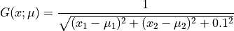
This function $G$ depends on the position $x=(x_1,x_2)\in\Omega=[0.1,0.9]^2$ in the 2D plane, and on the parameter $\mu=(\mu_1,\mu_2)\in\mathcal{D}=[-1,-0.01]^2$ of dimension 2 :

$G(x;\mu) = \frac{1}{\sqrt{(x_1 - \mu_1)^2 + (x_2 - \mu_2)^2 + 0.1^2}}$

The function is represented on a regular $\Omega_G$ spatial grid of size 20x20 points. It is available in ADAO built-in test models under the name TwoDimensionalInverseDistanceCS2010, together with the spatial and parametric domain default definition. So here we first build a set of simulations of $G$ for various $\mu$ parameter values, then we look for the best locations for measurements to obtain an DEIM interpolation representation of the fields, by applying the DEIM-type decomposition algorithm to it, and then derive some simple illustrations. 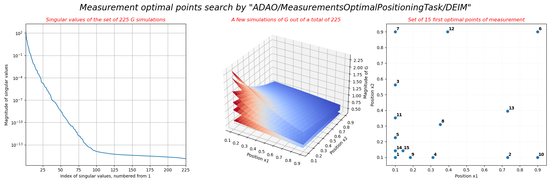We choose to look for an arbitrary number nbmeasures of 15 measurement locations.

It can be seen that the singular values decrease steadily down to numerical noise, indicating that around a hundred basis elements are needed to fully represent the information contained in the set of $G$ parametric simulations. Furthermore, the optimal measurement points in the $\Omega_G$ domain are inhomogeneously distributed, favoring the spatial zone near the $(0.1,0.1)$ corner in which the $G$ function varies more.

# -*- coding: utf-8 -*-
#
import numpy as np
import matplotlib.pyplot as plt
np.random.seed(123456789)
#
dimension = 20
nbmeasures = 15
#
print("Defining a set of artificial physical fields")
from Models.TwoDimensionalInverseDistanceCS2010 \
     import TwoDimensionalInverseDistanceCS2010 as Equation
Eq = Equation(dimension, dimension)
print()
#
print("Search for optimal measurement positions")
from adao import adaoBuilder
case = adaoBuilder.New()
case.setAlgorithmParameters(
    Algorithm = "MeasurementsOptimalPositioningTask",
    Parameters = {
        "Variant":"DEIM",
        "SampleAsnUplet":Eq.get_sample_of_mu(15, 15),
        "MaximumNumberOfLocations":nbmeasures,
        "ErrorNorm":"Linf",
        "ErrorNormTolerance":0.,
        "StoreSupplementaryCalculations":[
            "SingularValues",
            "OptimalPoints",
            "EnsembleOfSimulations",
            ],
        }
    )
case.setBackground(Vector = [1,1] )
case.setObservationOperator(OneFunction = Eq.OneRealisation)
case.execute()
#
#-------------------------------------------------------------------------------
print()
print("Graphical display of the results")
#
sp = case.get("EnsembleOfSimulations")[-1]
sv = case.get("SingularValues")[-1]
op = case.get("OptimalPoints")[-1]
#
x1, x2 = Eq.get_x()
x1, x2 = np.meshgrid(x1, x2)
posx1 = [x1.reshape((-1,))[ip] for ip in op]
posx2 = [x2.reshape((-1,))[ip] for ip in op]
Omega = Eq.get_bounds_on_space()
#
fig = plt.figure(figsize=(18, 6))
name = "Measurement optimal points search by "
name += '"ADAO/MeasurementsOptimalPositioningTask/DEIM"'
fig.suptitle(name, fontsize=20, fontstyle="italic")
#
ax = fig.add_subplot(1, 3, 1)
name = "Singular values of the set of %i G simulations"%sp.shape[1]
print("  -", name)
ax.set_title(name, fontstyle="italic", color="red")
ax.set_xlabel("Index of singular values, numbered from 1")
ax.set_ylabel("Magnitude of singular values")
ax.set_xlim(1, len(sv))
ax.set_yscale("log")
ax.grid(True)
ax.plot(range(1, 1 + len(sv)), sv)
#
ax = fig.add_subplot(1, 3, 2, projection = "3d")
name = "A few simulations of G out of a total of %i"%sp.shape[1]
print("  -", name)
ax.set_title(name, fontstyle="italic", color="red")
ax.set_xlabel("Position x1")
ax.set_ylabel("Position x2")
ax.set_zlabel("Magnitude of G")
for i in range(sp.shape[1]):
    if i % 44 != 0: continue
    Gfield = sp[:,i].reshape((dimension, dimension))
    ax.plot_surface(x1, x2, Gfield, cmap="coolwarm")
#
ax = fig.add_subplot(1, 3, 3)
name = "Set of %i first optimal points of measurement"%nbmeasures
print("  -", name)
ax.set_title(name, fontstyle="italic", color="red")
ax.set_xlabel("Position x1")
ax.set_ylabel("Position x2")
ax.set_xlim(Omega[0][0] - 0.05, Omega[0][1] + 0.05)
ax.set_ylim(Omega[1][0] - 0.05, Omega[1][1] + 0.05)
ax.grid(True, which="both", linestyle=(0, (1, 5)), linewidth=0.5)
ax.plot(posx1, posx2, markersize=6, marker="o", linestyle="")
for i in range(len(posx1)):
    ax.text(posx1[i] + 0.005, posx2[i] + 0.01, str(i + 1), fontweight="bold")
#
plt.tight_layout()
fig.savefig("simple_MeasurementsOptimalPositioningTask3.png")
plt.close()

The execution result is the following:

Defining a set of artificial physical fields

Search for optimal measurement positions

Graphical display of the results
  - Singular values of the set of 225 G simulations
  - A few simulations of G out of a total of 225
  - Set of 15 first optimal points of measurement

The figures illustrating the result of its execution are as follows:

_images/simple_MeasurementsOptimalPositioningTask3.png

15.3.6. See also¶

References to other sections:

Bibliographical references: