15.4. Task algorithm “ParameterCalibrationTask”¶

15.4.1. Description¶

This algorithm can be used to establish the calibration (or adjustment) of model parameters, based on observations or measurements and an a priori idea of these parameters.

It provides easy access to the most useful methods for such calibration. It is not intended to replace the other algorithms of data assimilation or optimization described elsewhere, but to accelerate the use of algorithms that are the most simple and the more efficient for parameter calibration. It also enables, when necessary, to initiate a calibration with the most classical methods, then very simply, by changing algorithm, to switch to more advanced specific methods or to those better adapted to the particular characteristics of the problems to be treated.

There are 4 main groups of methods which can be used to simply calibrate model parameters. The general conditions of choice are indicated here, with details available in each algorithm-specific section of the documentation.

3DVAR type variational optimization: variant “3DVARGradientOptimization”: The “3DVAR” gradient method is very often the most efficient, both because of the low number of calculations required and the high accuracy achieved. It requires good regularity of the model to be adjusted in relation to its parameters, good accuracy of the available simulations, and good separation of any possible equivalent minima. That said, when applied correctly, it is the most economical method in terms of model evaluations, and the most accurate for this number of evaluations. This is particularly true when the number of parameters to be optimized increases, a number to which the method is very un-sensitive. Last but not least, the method is easy to set up on a particular model, and requires little fine-tuning in order to assess its performance. For details and precise association of options, please refer to the specific documentation for a Calculation algorithm “3DVAR”.
BLUE type semi-linear estimation: variant “ExtendedBlueOptimization”: This is an “ExtendedBlue” estimation method, of BLUE (Best Linear Unbiased Estimator) type, which includes a non-linear evaluation of the model to be calibrated. The advantage of this method is that it’s a non-iterative estimate, and therefore very economical in terms of number of evaluations. What’s more, there are very few parameters to set when using this method. Nevertheless, by nature, it is usually less accurate and less robust to errors arising from the non-linear nature of the model used. For details and the precise association of options, please refer to the specific documentation for a Calculation algorithm “ExtendedBlue”.
Derivative free optimization: variant “DerivativeFreeOptimization”: It’s an optimization method that doesn’t use model derivation, but proceeds by simplex or other types of approximation. The advantage of this method is that it does not impose any particular behavior on the model in relation to its parameters. However, it often requires a large number of model evaluations to build an efficient approximation internally. Moreover, it is very sensitive to the number of parameters to be optimized, and is only suitable for low-dimensional models. The number of evaluations required is often several orders of magnitude greater than with other methods. Last but not least, parameter tuning is tricky on a particular model to be calibrated. For details and the precise association of options, please refer to the specific documentation for a Calculation algorithm “DerivativeFreeOptimization”.
Particle swarm optimization, canonical: variant “CanonicalParticuleSwarmOptimization”: This is a meta-heuristic optimization method, which uses a set (called a “swarm”) of model evaluations to map the state space and find the best one. The advantage of this method is that it is very insensitive to the number of parameters to be optimized, and seeks the global optimal state if possible, bearing in mind that parameter tuning is tricky on a particular model to calibrate. It is often one or two orders of magnitude more expensive than a variational method. For details and the precise association of options, please refer to the specific documentation for a Calculation algorithm “ParticleSwarmOptimization”.
Particle swarm optimization, accelerated: variant “VariationalParticuleSwarmOptimization”: This is a meta-heuristic optimization method enhanced by local search variational acceleration. If it can be applied, it ideally enables the global meta-heuristic swarm search to be combined with a local variational acceleration to overcome the difficulty of local swarm convergence. This method is more economical than the previous one in terms of the number of evaluations of the model to be calibrated, but it is rather tricky to tune to the given model to be calibrated. For details and the precise association of options, please refer to the specific documentation for a Calculation algorithm “ParticleSwarmOptimization”.

It is therefore recommended to keep the default variational optimization method “3DVARGradientOptimization” for the best possible performance, which offers also the easiest adjustment of the optimization parameters with respect to the model to calibrate.

15.4.2. Some noteworthy properties of the implemented methods¶

To complete the description, we summarize here a few notable properties of the algorithm methods or of their implementations. These properties may have an influence on how it is used or on its computational performance. For further information, please refer to the more comprehensive references given at the end of this algorithm description.

The methods proposed by this algorithm have internal parallelism, and can therefore take advantage of computational distribution resources. The potential interaction, between the parallelism of the numerical derivation, and the parallelism that may be present in the observation or evolution operators embedding user codes, must therefore be carefully tuned.

15.4.3. Optional and required commands¶

The general required commands, available in the editing user graphical or textual interface, are the following:

Background: Vector. The variable indicates the background or initial vector used, previously noted as $\mathbf{x}^b$ . Its value is defined as a “Vector” or “VectorSerie” type object. Its availability in output is conditioned by the boolean “Stored” associated with input.

BackgroundError: Matrix. This indicates the background error covariance matrix, previously noted as $\mathbf{B}$ . Its value is defined as a “Matrix” type object, a “ScalarSparseMatrix” type object, or a “DiagonalSparseMatrix” type object, as described in detail in the section Requirements to describe covariance matrices. Its availability in output is conditioned by the boolean “Stored” associated with input.

EvolutionError: Matrix. The variable indicates the evolution error covariance matrix, usually noted as $\mathbf{Q}$ . It is defined as a “Matrix” type object, a “ScalarSparseMatrix” type object, or a “DiagonalSparseMatrix” type object, as described in detail in the section Requirements to describe covariance matrices. Its availability in output is conditioned by the boolean “Stored” associated with input.

EvolutionModel: Operator. The variable indicates the evolution model operator, usually noted $M$ , which describes an elementary step of evolution. Its value is defined as a “Function” type object or a “Matrix” type one. In the case of “Function” type, different functional forms can be used, as described in the section Requirements for functions describing an operator. If there is some control $U$ included in the evolution model, the operator has to be applied to a pair $(X,U)$ .

Observation: List of vectors. The variable indicates the observation vector used for data assimilation or optimization, and usually noted $\mathbf{y}^o$ . Its value is defined as an object of type “Vector” if it is a single observation (temporal or not) or “VectorSeries” if it is a succession of observations. Its availability in output is conditioned by the boolean “Stored” associated in input.

ObservationError: Matrix. The variable indicates the observation error covariance matrix, usually noted as $\mathbf{R}$ . It is defined as a “Matrix” type object, a “ScalarSparseMatrix” type object, or a “DiagonalSparseMatrix” type object, as described in detail in the section Requirements to describe covariance matrices. Its availability in output is conditioned by the boolean “Stored” associated with input.

ObservationOperator: Operator. The variable indicates the observation operator, usually noted as $H$ , which transforms the input parameters $\mathbf{x}$ to results $\mathbf{y}$ to be compared to observations $\mathbf{y}^o$ . Its value is defined as a “Function” type object or a “Matrix” type one. In the case of “Function” type, different functional forms can be used, as described in the section Requirements for functions describing an operator. If there is some control $U$ included in the observation, the operator has to be applied to a pair $(X,U)$ .

The general optional commands, available in the editing user graphical or textual interface, are indicated in List of commands and keywords for a dedicated task or study oriented case. Moreover, the parameters of the command “AlgorithmParameters” allow to choose the specific options, described hereafter, of the algorithm. See Description of options of an algorithm by “AlgorithmParameters” for the good use of this command.

The options are the following:

It should be noted that all the options available for this task are described here, but that only some are active for a particular variant. The precise documentation of each variant is therefore also useful for the correct use of each of the options presented here.

Bounds

List of pairs of real values. This key allows to define pairs of upper and lower bounds for every state variable being optimized. Bounds have to be given by a list of list of pairs of lower/upper bounds for each variable, with a value of None each time there is no bound. The bounds can always be specified, but they are taken into account only by the constrained optimizers. If the list is empty, there are no bounds.

Example: {"Bounds":[[2.,5.],[1.e-2,10.],[-30.,None],[None,None]]}

CognitiveAcceleration

Real value. This key indicates the recall rate at the best previously known value of the current insect’s history. It is a floating point positive value. The default value is about $1/2+ln(2)=1.19315$ , and it is recommended to adapt it, rather by reducing it, to the physical case that is being treated.

In the standard (non-adaptive) case, this rate is constant and is equal to the indicated value. In the ASAPSO adaptive case [Wang09], the value of this key indicates the initial recall rate, which then decreases linearly with the number of generations and the associated “CognitiveAccelerationControl” factor.

Example : {"CognitiveAcceleration":1.19315}

CognitiveAccelerationControl

Real value. This key indicates the factor of change in the recall rate towards the best previously known value of the current insect’s history. It is a positive real value whose default is 0, that is, by default, there is no change in the recall rate.

In the ASAPSO adaptive case [Wang09], the value of this key indicates the linear decrease factor of the recall rate with the number of generations (with respect to the requested total number of generations), given that the initial value of the rate is indicated by the associated “CognitiveAcceleration” factor. There is no recommended value, but you could, for example, use the initial value $1.19315$ of the associated factor if you want to cancel any recall towards the best known value of the history at the end of the iterations.

Example : {"CognitiveAccelerationControl":0.}

CostDecrementTolerance

Real value. This key indicates a limit value, leading to stop successfully the iterative optimization process when the cost function decreases less than this tolerance at the last step. The default is 1.e-7, and it is recommended to adapt it to the needs on real problems. One can refer to the section describing ways for Convergence control for calculation cases and iterative algorithms for more detailed recommendations.

Example: {"CostDecrementTolerance":1.e-7}

DistributionByComponents

List of predefined names. This keyword only needs to be defined when the particle swarm initialization for the “ParticleSwarmOptimization” algorithm is set to “DistributionByComponents”. In this case, for each state component, the chosen distribution must be indicated in the form of a predefined name. Possible names are “uniform”, “loguniform”, “logarithmic”, “[‘normal’,σ]”, “[‘lognormal’,σ]” and “[‘logarithmicnormal’,σ]”. All “normal” distributions must be accompanied by an indication of the standard deviation σ, given that they are centered in the definition domain. The values “uniform”, “loguniform”, “normal”, “lognormal” only affect position initialization by applying the indicated distribution, while the values “logarithmic” and “logarithmicnormal” affect both position and motion initialization. There must be the same number of values indicated as the size of an individual state. Distributions conform to the limits specified for the “*ParticleSwarmOptimization” algorithm. Distributions can be different for each axis. When an identical distribution is chosen for all components, this is equivalent to choosing the global value of the previous keyword instead, if it exists.

Example : {"DistributionByComponents" : ['uniform', 'loguniform', 'logarithmic', ['normal', 1]]} for a state space of dimension 4.

GlobalCostReductionTolerance

Real value. This key indicates the limit reduction factor, leading to the iterative optimization process being stopped when the cost function decreases by at least this tolerance over the entire optimal search. The default value is 1.e-16 (equivalent to no effect), and it is recommended to adapt it to the needs of real problems.

Example: {"GlobalCostReductionTolerance":1.e-16}

GradientNormTolerance

Real value. This key indicates a limit value, leading to stop successfully the iterative optimization process when the norm of the gradient is under this limit. It is only used for non-constrained optimizers. The default is 1.e-5 and it is not recommended to change it.

Example: {"GradientNormTolerance":1.e-5}

HybridCostDecrementTolerance

Real value. This key indicates a limit value, leading to stop successfully the optimization process for the variational part in the coupling, when the cost function decreases less than this tolerance at the last step. The default is 1.e-7, and it is recommended to adapt it to the needs on real problems. One can refer to the section describing ways for Convergence control for calculation cases and iterative algorithms for more detailed recommendations.

Example: {"HybridCostDecrementTolerance":1.e-7}

HybridMaximumNumberOfIterations

Integer value. This key indicates the maximum number of internal iterations allowed for hybrid optimization, for the variational part. The default is 15000, which is very similar to no limit on iterations. It is then recommended to adapt this parameter to the needs on real problems. For some optimizers, the effective stopping step can be slightly different of the limit due to algorithm internal control requirements. One can refer to the section describing ways for Convergence control for calculation cases and iterative algorithms for more detailed recommendations.

Example: {"HybridMaximumNumberOfIterations":100}

HybridNumberOfLocalHunters

Integer value. This key indicates the number of insects on which the local search will be conducted. Insects are chosen as the best from the current iteration of the global search. With a default value of 1, the local search is performed on the best insect only. It is then recommended to adapt this parameter to the needs on real problems.

Example : {"HybridNumberOfLocalHunters":1}

HybridNumberOfWarmupIterations

Integer value. This key indicates the number of initial iterations of the global search performed before establishing a local search on the best insects. By default, with a value of 0, the local search is performed from the first iterative step of the global search.

Example : {"HybridNumberOfWarmupIterations":0}

InertiaWeight

Real value. This key indicates the part of the insect velocity which is imposed by the swarm, named “inertia weight”. It is a positive floating point value. It is a floating point value between 0 and 1. The default value is about $1/(2*ln(2))$ and it is recommended to adapt it to the physical case that is being treated.

Example : {"InertiaWeight":0.72135}

InitializationPoint

Vector. The variable specifies one vector to be used as the initial state around which an iterative algorithm starts. By default, this initial state is not required and is equal to the background $\mathbf{x}^b$ . Its value must allow to build a vector of the same size as the background. If provided, it replaces the background only for initialization.

Example : {"InitializationPoint":[1, 2, 3, 4, 5]}

MaximumNumberOfFunctionEvaluations

Integer value. This key indicates the maximum number of evaluation of the cost function to be optimized. The default is 15000, which is an arbitrary limit. It is then recommended to adapt this parameter to the needs on real problems. For some optimizers, the effective number of function evaluations can be slightly different of the limit due to algorithm internal control requirements.

Example: {"MaximumNumberOfFunctionEvaluations":50}

MaximumNumberOfIterations

Integer value. This key indicates the maximum number of internal iterations allowed for iterative optimization. The default is 15000, which is very similar to no limit on iterations. It is then recommended to adapt this parameter to the needs on real problems. For some optimizers, the effective stopping step can be slightly different of the limit due to algorithm internal control requirements. One can refer to the section describing ways for Convergence control for calculation cases and iterative algorithms for more detailed recommendations.

Example: {"MaximumNumberOfIterations":100}

Minimizer

Predefined name. This key allows to choose the optimization minimizer. The default choice is “LBFGSB”, and the possible ones for variational variants are “LBFGSB” (nonlinear constrained minimizer, see [Byrd95], [Morales11], [Zhu97]), “BFGS” (nonlinear unconstrained minimizer), and the following ones for variants without derivation are “BOBYQA” (minimization, with or without constraints, by quadratic approximation, see [Powell09]), “COBYLA” (minimization, with or without constraints, by linear approximation, see [Powell94] [Powell98]). “NEWUOA” (minimization, with or without constraints, by iterative quadratic approximation, see [Powell04]), “POWELL” (minimization, unconstrained, using conjugate directions, see [Powell64]), “SIMPLEX” (minimization, with or without constraints, using Nelder-Mead simplex algorithm, see [Nelder65] and [WikipediaNM]), “SUBPLEX” (minimization, with or without constraints, using Nelder-Mead simplex algorithm on a sequence of subspaces, see [Rowan90]). Only the “POWELL” minimizer does not allow to deal with boundary constraints, all the others take them into account if they are present in the case definition.

Example : {"Minimizer":"LBFGSB"}

NumberOfInsects

Integer value. This key indicates the number of insects or particles in the swarm. The default is 100, which is a usual default for this algorithm.

Example : {"NumberOfInsects":100}

NumberOfSamplesForQuantiles

Integer value. This key indicates the number of simulation to be done in order to estimate the quantiles. This option is useful only if the supplementary calculation “SimulationQuantiles” has been chosen. The default is 100, which is often sufficient for correct estimation of common quantiles at 5%, 10%, 90% or 95%.

Example: {"NumberOfSamplesForQuantiles":100}

ProjectedGradientTolerance

Real value. This key indicates a limit value, leading to stop successfully the iterative optimization process when all the components of the projected gradient are under this limit. It is only used for constrained optimizers. The default is -1, that is the internal default of each minimizer (generally 1.e-5), and it is not recommended to change it.

Example: {"ProjectedGradientTolerance":-1}

QualityCriterion

Predefined name. This key indicates the quality criterion, minimized to find the optimal state estimate. The default is the usual data assimilation criterion named “DA”, the augmented weighted least squares. The possible criterion has to be in the following list, where the equivalent names are indicated by the sign “<=>”: [“AugmentedWeightedLeastSquares” <=> “AWLS” <=> “DA”, “WeightedLeastSquares” <=> “WLS”, “LeastSquares” <=> “LS” <=> “L2”, “AbsoluteValue” <=> “L1”, “MaximumError” <=> “ME” <=> “Linf”]. See the section for Going further in the state estimation by optimization methods to have a detailed definition of these quality criteria.

Example: {"QualityCriterion":"DA"}

Quantiles

List of real values. This list indicates the values of quantile, between 0 and 1, to be estimated by simulation around the optimal state. The sampling uses a multivariate Gaussian random sampling, directed by the a posteriori covariance matrix. This option is useful only if the supplementary calculation “SimulationQuantiles” has been chosen. The default is a void list.

Example: {"Quantiles":[0.1,0.9]}

SetSeed

Integer value. This key allow to give an integer in order to fix the seed of the random generator used in the algorithm. By default, the seed is left uninitialized, and so use the default initialization from the computer, which then change at each study. To ensure the reproducibility of results involving random samples, it is strongly advised to initialize the seed. A simple convenient value is for example 123456789. It is recommended to put an integer with more than 6 or 7 digits to properly initialize the random generator.

Example: {"SetSeed":123456789}

SimulationForQuantiles

Predefined name. This key indicates the type of simulation, linear (with the tangent observation operator applied to perturbation increments around the optimal state) or non-linear (with standard observation operator applied to perturbed states), one want to do for each perturbation. It changes mainly the time of each elementary calculation, usually longer in non-linear than in linear. This option is useful only if the supplementary calculation “SimulationQuantiles” has been chosen. The default value is “Linear”, and the possible choices are “Linear” and “NonLinear”.

Example: {"SimulationForQuantiles":"Linear"}

SocialAcceleration

Real value. This key indicates the recall rate towards the best insect in the current insect’s neighborhood, which by default is the complete swarm. It is a floating point positive value. The default value is about $1/2+ln(2)=1.19315$ and it is recommended to adapt it, rather by reducing it, to the physical case that is being treated.

In the standard (non-adaptive) case, this rate is constant and is equal to the indicated value. In the ASAPSO adaptive case [Wang09], the value of this key indicates the initial recall rate, which then increases linearly with the number of generations and the associated “SocialAccelerationControl” factor.

Example : {"SocialAcceleration":1.19315}

SocialAccelerationControl

Real value. This key indicates the factor of change in the recall rate towards the best insect in the current insect’s neighborhood, which by default is the complete swarm. It is a positive real value whose default is 0, that is, by default, there is no change in the recall rate.

In the ASAPSO adaptive case [Wang09], the value of this key indicates the linear growth factor of the recall rate with the number of generations ( with respect to the requested total number of generations), given that the initial value of the rate is indicated by the associated “SocialAcceleration” factor. There is no recommended value, but you can use the initial value $1.19315$ of the associated factor, for example, if you want to double the recall towards the best known value of the neighborhood at the end of the iterations.

Example : {"SocialAccelerationControl":0.}

StateBoundsForQuantiles

List of pairs of real values. This key allows to define pairs of upper and lower bounds for every state variable used for quantile simulations. Bounds have to be given by a list of list of pairs of lower/upper bounds for each variable, with possibly None every time there is no bound.

If these bounds are not defined for quantile simulation and if optimization bounds are defined, they are used for quantile simulation. If these bounds for quantile simulation are defined, they are used regardless of the optimization bounds defined. If this variable is set to None, then no bounds are used for the states used in the quantile simulation regardless of the optimization bounds defined.

Example : {"StateBoundsForQuantiles":[[2.,5.],[1.e-2,10.],[-30.,None],[None,None]]}

StateVariationTolerance

Real value. This key indicates the maximum relative variation of the state for stopping by convergence on the state. The default is 1.e-4, and it is recommended to adapt it to the needs on real problems.

Example: {"StateVariationTolerance":1.e-4}

StoreSupplementaryCalculations

List of names. This list indicates the names of the supplementary variables, that can be available during or at the end of the algorithm, if they are initially required by the user. Their availability involves, potentially, costly calculations or memory consumptions. The default is then a void list, none of these variables being calculated and stored by default (excepted the unconditional variables). The possible names are in the following list (the detailed description of each named variable is given in the following part of this specific algorithmic documentation, in the sub-section “Information and variables available at the end of the algorithm”): [ “Analysis”, “APosterioriCorrelations”, “APosterioriCovariance”, “APosterioriStandardDeviations”, “APosterioriVariances”, “BMA”, “CostFunctionJ”, “CostFunctionJAtCurrentOptimum”, “CostFunctionJb”, “CostFunctionJbAtCurrentOptimum”, “CostFunctionJo”, “CostFunctionJoAtCurrentOptimum”, “CurrentIterationNumber”, “CurrentOptimum”, “CurrentState”, “CurrentStepNumber”, “EnsembleOfSimulations”, “EnsembleOfStates”, “ForecastState”, “IndexOfOptimum”, “Innovation”, “InnovationAtCurrentAnalysis”, “InnovationAtCurrentState”, “JacobianMatrixAtBackground”, “JacobianMatrixAtOptimum”, “KalmanGainAtOptimum”, “MahalanobisConsistency”, “OMA”, “OMB”, “SampledStateForQuantiles”, “SigmaObs2”, “SimulatedObservationAtBackground”, “SimulatedObservationAtCurrentOptimum”, “SimulatedObservationAtCurrentState”, “SimulatedObservationAtOptimum”, “SimulationQuantiles”, ].

Example : {"StoreSupplementaryCalculations":["CurrentState", "Residu"]}

SwarmInitialization

Predefined name. The name defines the particle swarm initialization mode for the “ParticleSwarmOptimization” algorithm. The particle series is initialized by specifying the distribution per component, which can be identical for all components (this is the case for all values except “DistributionByComponents”), or component-specific with “DistributionByComponents”. In the latter case, it is also necessary to specify the “DistributionByComponents” keyword content. The default value is “UniformByComponents”.

The possible name is therefore in the following list: [“UniformByComponents”, “LogUniformByComponents”, “LogarithmicByComponents”, “DistributionByComponents”].

Example : {"SwarmInitialization":"UniformByComponents"}

SwarmTopology

Predefined name. This key indicates how the particles (or insects) communicate information to each other during the evolution of the particle swarm. The most classical method consists in exchanging information between all particles (called “gbest” or “FullyConnectedNeighborhood”). But it is often more efficient to exchange information on a reduced neighborhood, as in the classical method “lbest” (or “RingNeighborhoodWithRadius1”) exchanging information with the two neighboring particles in numbering order (the previous one and the next one), or the method “RingNeighborhoodWithRadius2” exchanging with the 4 neighbors (the two previous ones and the two following ones). A variant of reduced neighborhood consists in exchanging with 3 neighbors (method “AdaptativeRandomWith3Neighbors”) or 5 neighbors (method “AdaptativeRandomWith5Neighbors”) chosen randomly (the particle can be drawn several times). The default value is “FullyConnectedNeighborhood”, and it is advisable to change it carefully depending on the properties of the simulated physical system. The possible communication topology is to be chosen from the following list, in which the equivalent names are indicated by a “<=>” sign: [“FullyConnectedNeighborhood” <=> “FullyConnectedNeighbourhood” <=> “gbest”, “RingNeighborhoodWithRadius1” <=> “RingNeighbourhoodWithRadius1” <=> “lbest”, “RingNeighborhoodWithRadius2” <=> “RingNeighbourhoodWithRadius2”, “AdaptativeRandomWith3Neighbors” <=> “AdaptativeRandomWith3Neighbours” <=> “abest”, “AdaptativeRandomWith5Neighbors” <=> “AdaptativeRandomWith5Neighbours”].

Example : {"SwarmTopology":"FullyConnectedNeighborhood"}

VelocityClampingFactor

Real value. This key indicates the rate of group velocity attenuation in the update for each insect, useful to avoid swarm explosion, i.e. uncontrolled growth of insect velocity. It is a floating point value between 0+ and 1. The default value is 0.3.

Example : {"VelocityClampingFactor":0.3}

Variant

Predefined name. This key allows to choose one of the possible variants for the main calibration algorithm. The default variant is the original “3DVAR”, and the possible choices are “3DVARGradientOptimization” or “3DVAR” (3DVAR type variational analysis), “ExtendedBlueOptimization” or “ExtendedBlue” (BLUE type semi-linear estimation), “DerivativeFreeOptimization” or “DFO” (derivative-free optimization using simplex or other approximations), “CanonicalParticuleSwarmOptimization” or “CanonicalPSO” ou “PSO” (canonical particle swarm optimization), “VariationalParticuleSwarmOptimization” or “SPSO-2011-AIS-VLS” (2011 standard particle swarm optimization, accelerated by local variational search), It is highly recommended to keep the default value.

Example : {"Variant":"3DVAR"}

15.4.4. Information and variables available at the end of the algorithm¶

At the output, after executing the algorithm, there are information and variables originating from the calculation. The description of Variables and information available at the output show the way to obtain them by the method named get, of the variable “ADD” of the post-processing in graphical interface, or of the case in textual interface. The input variables, available to the user at the output in order to facilitate the writing of post-processing procedures, are described in an Inventory of potentially available information at the output.

Permanent outputs (non conditional)

The unconditional outputs of the algorithm are the following:

Analysis

List of vectors. Each element of this variable is an optimal state $\mathbf{x}^*$ in optimization, an interpolate or an analysis $\mathbf{x}^a$ in data assimilation.

Example: xa = ADD.get("Analysis")[-1]

CostFunctionJ

List of values. Each element is a value of the chosen error function $J$ .

Example: J = ADD.get("CostFunctionJ")[:]

CostFunctionJb

List of values. Each element is a value of the error function $J^b$ , that is of the background difference part. If this part does not exist in the error function, its value is zero.

Example: Jb = ADD.get("CostFunctionJb")[:]

CostFunctionJo

List of values. Each element is a value of the error function $J^o$ , that is of the observation difference part.

Example: Jo = ADD.get("CostFunctionJo")[:]

CurrentState

List of vectors. Each element is a usual state vector used during the iterative algorithm procedure.

Example: xs = ADD.get("CurrentState")[:]

Set of on-demand outputs (conditional or not)

The whole set of algorithm outputs (conditional or not), sorted by alphabetical order, is the following:

Analysis

List of vectors. Each element of this variable is an optimal state $\mathbf{x}^*$ in optimization, an interpolate or an analysis $\mathbf{x}^a$ in data assimilation.

Example: xa = ADD.get("Analysis")[-1]

APosterioriCorrelations

List of matrices. Each element is an a posteriori error correlations matrix of the optimal state, coming from the $\mathbf{A}$ covariance matrix. In order to get them, this a posteriori error covariances calculation has to be requested at the same time.

Example: apc = ADD.get("APosterioriCorrelations")[-1]

APosterioriCovariance

List of matrices. Each element is an a posteriori error covariance matrix $\mathbf{A}$ of the optimal state.

Example: apc = ADD.get("APosterioriCovariance")[-1]

APosterioriStandardDeviations

List of matrices. Each element is an a posteriori error standard errors diagonal matrix of the optimal state, coming from the $\mathbf{A}$ covariance matrix. In order to get them, this a posteriori error covariances calculation has to be requested at the same time.

Example: aps = ADD.get("APosterioriStandardDeviations")[-1]

APosterioriVariances

List of matrices. Each element is an a posteriori error variance errors diagonal matrix of the optimal state, coming from the $\mathbf{A}$ covariance matrix. In order to get them, this a posteriori error covariances calculation has to be requested at the same time.

Example: apv = ADD.get("APosterioriVariances")[-1]

BMA

List of vectors. Each element is a vector of difference between the background and the optimal state.

Example: bma = ADD.get("BMA")[-1]

CostFunctionJ

List of values. Each element is a value of the chosen error function $J$ .

Example: J = ADD.get("CostFunctionJ")[:]

CostFunctionJAtCurrentOptimum

List of values. Each element is a value of the error function $J$ . At each step, the value corresponds to the optimal state found from the beginning.

Example: JACO = ADD.get("CostFunctionJAtCurrentOptimum")[:]

CostFunctionJb

List of values. Each element is a value of the error function $J^b$ , that is of the background difference part. If this part does not exist in the error function, its value is zero.

Example: Jb = ADD.get("CostFunctionJb")[:]

CostFunctionJbAtCurrentOptimum

List of values. Each element is a value of the error function $J^b$ . At each step, the value corresponds to the optimal state found from the beginning. If this part does not exist in the error function, its value is zero.

Example: JbACO = ADD.get("CostFunctionJbAtCurrentOptimum")[:]

CostFunctionJo

List of values. Each element is a value of the error function $J^o$ , that is of the observation difference part.

Example: Jo = ADD.get("CostFunctionJo")[:]

CostFunctionJoAtCurrentOptimum

List of values. Each element is a value of the error function $J^o$ , that is of the observation difference part. At each step, the value corresponds to the optimal state found from the beginning.

Example: JoACO = ADD.get("CostFunctionJoAtCurrentOptimum")[:]

CurrentIterationNumber

List of integers. Each element is the iteration index at the current step during the iterative algorithm procedure. There is one iteration index value per assimilation step corresponding to an observed state.

Example: cin = ADD.get("CurrentIterationNumber")[-1]

CurrentOptimum

List of vectors. Each element is the optimal state obtained at the usual step of the iterative algorithm procedure of the optimization algorithm. It is not necessarily the last state.

Example: xo = ADD.get("CurrentOptimum")[:]

CurrentState

List of vectors. Each element is a usual state vector used during the iterative algorithm procedure.

Example: xs = ADD.get("CurrentState")[:]

CurrentStepNumber

List of integers. Each element is the index of the current step in the iterative process, driven by the series of observations, of the algorithm used. This corresponds to the observation step used. Note: it is not the index of the current iteration of the algorithm even if it coincides for non-iterative algorithms.

Example: csn = ADD.get("CurrentStepNumber")[-1]

EnsembleOfSimulations

List of vectors or matrix. This key contains an ordered collection of physical state vectors or simulated state vectors $\mathbf{y}$ that may be observed. These are $H$ operator outputs, i.e. simulated observation states (called “snapshots” in reduced-base terminology). At each step index, there is 1 state per column if this list is in matrix form, or 1 state per element if it’s actually a list. Caution: the numbering of the support or points, on which or to which a state value is given in each vector, is implicitly that of the natural order of numbering of the state vector, from 0 to the “size minus 1” of this vector.

Example : {"EnsembleOfSimulations":[y1, y2, y3...]}

EnsembleOfStates

List of vectors or matrix. Each element is an ordered collection of physical or parameter state vectors $\mathbf{x}$ . These are $H$ operator entries, i.e. current states before observation. At each step index, there is 1 state per column if this list is in matrix form, or 1 state per element if it’s actually a list. Caution: the numbering of the support or points, on which or to which a state value is given in each vector, is implicitly that of the natural order of numbering of the state vector, from 0 to the “size minus 1” of this vector.

Example : {"EnsembleOfStates":[x1, x2, x3...]}

ForecastState

List of vectors. Each element is a state vector forecasted by the model during the iterative algorithm procedure.

Example: xf = ADD.get("ForecastState")[:]

IndexOfOptimum

List of integers. Each element is the iteration index of the optimum obtained at the current step of the iterative algorithm procedure of the optimization algorithm. It is not necessarily the number of the last iteration.

Example: ioo = ADD.get("IndexOfOptimum")[-1]

Innovation

List of vectors. Each element is an innovation vector, which is in static the difference between the optimal and the background, and in dynamic the evolution increment.

Example: d = ADD.get("Innovation")[-1]

InnovationAtCurrentAnalysis

List of vectors. Each element is an innovation vector at current analysis. This quantity is identical to the innovation vector at analysed state in the case of a single-state assimilation.

Example: da = ADD.get("InnovationAtCurrentAnalysis")[-1]

InnovationAtCurrentState

List of vectors. Each element is an innovation vector at current state before analysis.

Example: ds = ADD.get("InnovationAtCurrentState")[-1]

JacobianMatrixAtBackground

List of matrices. Each element is the jacobian matrix of partial derivatives of the output of the observation operator with respect to the input parameters, one column of derivatives per parameter. It is calculated at the initial state.

Example: gradh = ADD.get("JacobianMatrixAtBackground")[-1]

JacobianMatrixAtOptimum

List of matrices. Each element is the jacobian matrix of partial derivatives of the output of the observation operator with respect to the input parameters, one column of derivatives per parameter. It is calculated at the optimal state.

Example: gradh = ADD.get("JacobianMatrixAtOptimum")[-1]

KalmanGainAtOptimum

List of matrices. Each element is a standard Kalman gain matrix, evaluated using the linearized observation operator. It is calculated at the optimal state.

Example: kg = ADD.get("KalmanGainAtOptimum")[-1]

MahalanobisConsistency

List of values. Each element is a value of the Mahalanobis quality indicator.

Example: mc = ADD.get("MahalanobisConsistency")[-1]

OMA

List of vectors. Each element is a vector of difference between the observation and the optimal state in the observation space.

Example: oma = ADD.get("OMA")[-1]

OMB

List of vectors. Each element is a vector of difference between the observation and the background state in the observation space.

Example: omb = ADD.get("OMB")[-1]

SampledStateForQuantiles

List of vector series. Each element is a series of column state vectors, generated to estimate by simulation and/or observation the quantile values required by the user. There are as many states as the number of samples required for this quantile estimate.

Example : xq = ADD.get("SampledStateForQuantiles")[:]

SigmaObs2

List of values. Each element is a value of the quality indicator $(\sigma^o)^2$ of the observation part.

Example: so2 = ADD.get("SigmaObs")[-1]

SimulatedObservationAtBackground

List of vectors. Each element is a vector of observation simulated by the observation operator from the background $\mathbf{x}^b$ . It is the forecast from the background, and it is sometimes called “Dry”.

Example: hxb = ADD.get("SimulatedObservationAtBackground")[-1]

SimulatedObservationAtCurrentOptimum

List of vectors. Each element is a vector of observation simulated from the optimal state obtained at the current step the optimization algorithm, that is, in the observation space.

Example: hxo = ADD.get("SimulatedObservationAtCurrentOptimum")[-1]

SimulatedObservationAtCurrentState

List of vectors. Each element is an observed vector simulated by the observation operator from the current state, that is, in the observation space.

Example: hxs = ADD.get("SimulatedObservationAtCurrentState")[-1]

SimulatedObservationAtOptimum

List of vectors. Each element is a vector of observation obtained by the observation operator from simulation on the analysis or optimal state $\mathbf{x}^a$ . It is the observed forecast from the analysis or the optimal state, and it is sometimes called “Forecast”.

Example: hxa = ADD.get("SimulatedObservationAtOptimum")[-1]

SimulationQuantiles

List of vector series. Each element is a series of observation column vectors, corresponding, for a particular quantile required by the user, to the observed state that achieves the requested quantile. Each observation column vector is rendered in the same order as the quantile values required by the user.

Example: sQuantiles = ADD.get("SimulationQuantiles")[:]

15.4.5. Python (TUI) use examples¶

Here is one or more very simple examples of the proposed algorithm and its parameters, written in [DocR] Textual User Interface for ADAO (TUI/API). Moreover, when it is possible, the information given as input also allows to define an equivalent case in [DocR] Graphical User Interface for ADAO (GUI/EFICAS).

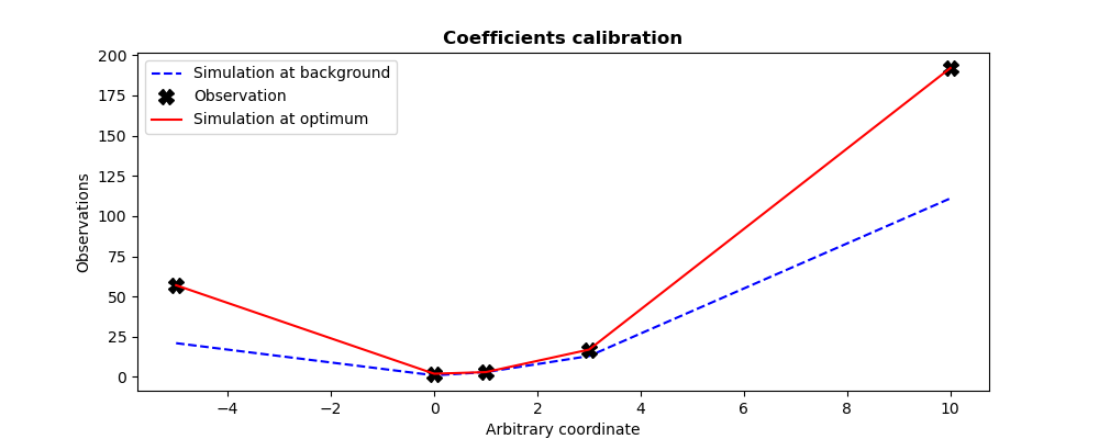
15.4.5.1. First example¶

This example describes the calibration of parameters $\mathbf{x}$ of a quadratic observation model $H$ . This model $H$ is here represented as a function named QuadFunction for the purpose of this example. This function get as input the coefficients vector $\mathbf{x}$ of the quadratic form, and return as output the evaluation vector $\mathbf{y}$ of the quadratic model at the predefined internal control points, predefined in a static way in the model.

The calibration is done using an initial coefficient set (background state specified by Xb in the example), and with the information $\mathbf{y}^o$ (specified by Yobs in the example) of 5 measures obtained in these same internal control points. We set twin experiments (see To test a data assimilation chain: the twin experiments) and the measurements are supposed to be perfect. We choose to emphasize the observations, versus the background, by setting artificially a great variance for the background error, here of $10^{6}$ .

A 3DVAR variational optimization is used (default method), explicitly requested here by the “3DVARGradientOptimization” variant specified for this algorithm. By nature, the same results are obtained as in the first “3DVAR” algorithme example (see its Python (TUI) use examples).

# -*- coding: utf-8 -*-
#
from numpy import array, ravel, abs, max, set_printoptions
set_printoptions(precision=7)
def QuadFunction( coefficients ):
    """
    Quadratic simulation in x points: y = a x^2 + b x + c
    """
    a, b, c = list(ravel(coefficients))
    x_points = (-5, 0, 1, 3, 10)
    y_points = []
    for x in x_points:
        y_points.append( a*x*x + b*x + c )
    return array(y_points)
#
Xb   = array([1., 1., 1.])
Yobs = array([57, 2, 3, 17, 192])
#
from adao import adaoBuilder
case = adaoBuilder.New()
case.setBackground( Vector = Xb, Stored=True )
case.setBackgroundError( ScalarSparseMatrix = 1.e6 )
case.setObservation( Vector = Yobs, Stored=True )
case.setObservationError( ScalarSparseMatrix = 1. )
case.setObservationOperator( OneFunction = QuadFunction )
case.setAlgorithmParameters(
    Algorithm="ParameterCalibrationTask",
    Parameters={
        "Variant":"3DVARGradientOptimization",
        "Minimizer":"LBFGSB",
        "MaximumNumberOfIterations": 100,
        "StoreSupplementaryCalculations": [
            "CurrentState",
            "OMA",
            ],
        },
    )
case.execute()
#
#-------------------------------------------------------------------------------
#
print("Calibration of %i coefficients in a 1D quadratic function on %i measures"%(
    len(case.get("Background")),
    len(case.get("Observation")),
    ))
print("----------------------------------------------------------------------")
print("")
print("Observation vector.................:", ravel(case.get("Observation")))
print("A priori background state..........:", ravel(case.get("Background")))
print("")
print("Expected theoretical coefficients..:", ravel((2,-1,2)))
print("")
print("Number of simulations..............:", len(case.get("CurrentState"))*4)
print("Maximum diff. Observation-Analyse..:", "%.2e"%max(abs(ravel(case.get("OMA")[-1]))))
print("Calibration resulting coefficients.:", ravel(case.get("Analysis")[-1]))
#
Xa = case.get("Analysis")[-1]
import matplotlib.pyplot as plt
plt.rcParams["figure.figsize"] = (10, 4)
#
plt.figure()
plt.plot((-5,0,1,3,10),QuadFunction(Xb),"b--",label="Simulation at background")
plt.plot((-5,0,1,3,10),Yobs,            "kX", label="Observation",markersize=10)
plt.plot((-5,0,1,3,10),QuadFunction(Xa),"r-", label="Simulation at optimum")
plt.legend()
plt.title("Coefficients calibration", fontweight="bold")
plt.xlabel("Arbitrary coordinate")
plt.ylabel("Observations")
plt.savefig("simple_ParameterCalibrationTask1.png")

The execution result is the following:

Calibration of 3 coefficients in a 1D quadratic function on 5 measures
----------------------------------------------------------------------

Observation vector.................: [ 57.   2.   3.  17. 192.]
A priori background state..........: [1. 1. 1.]

Expected theoretical coefficients..: [ 2 -1  2]

Number of simulations..............: 100
Maximum diff. Observation-Analyse..: 5.83e-07
Calibration resulting coefficients.: [ 2.        -0.9999999  1.9999999]

The figures illustrating the result of its execution are as follows:

_images/simple_ParameterCalibrationTask1.png

15.4.5.2. Second example¶

Since it’s easy to change optimization approach, the aim of this second example is to calibrate parameters using derivative-free optimization. This is indicated to this algorithm by the variant “DerivativeFreeOptimization” (accompanied by a change of optimizer by the keyword “Minimizer”). Only the values of these two keywords “Variant” and “Minimizer” therefore change between the two approaches.

In this extremely simple case, of small dimensions and without any special optimization difficulty, the control parameters remain the same. The results are of the same quality as for the reference variational optimization.

# -*- coding: utf-8 -*-
#
from numpy import array, ravel, abs, max, set_printoptions
set_printoptions(precision=7)
def QuadFunction( coefficients ):
    """
    Quadratic simulation in x points: y = a x^2 + b x + c
    """
    a, b, c = list(ravel(coefficients))
    x_points = (-5, 0, 1, 3, 10)
    y_points = []
    for x in x_points:
        y_points.append( a*x*x + b*x + c )
    return array(y_points)
#
Xb   = array([1., 1., 1.])
Yobs = array([57, 2, 3, 17, 192])
#
from adao import adaoBuilder
case = adaoBuilder.New()
case.setBackground( Vector = Xb, Stored=True )
case.setBackgroundError( ScalarSparseMatrix = 1.e6 )
case.setObservation( Vector = Yobs, Stored=True )
case.setObservationError( ScalarSparseMatrix = 1. )
case.setObservationOperator( OneFunction = QuadFunction )
case.setAlgorithmParameters(
    Algorithm="ParameterCalibrationTask",
    Parameters={
        "Variant":"DerivativeFreeOptimization",
        "Minimizer":"BOBYQA",
        "MaximumNumberOfIterations": 100,
        "StoreSupplementaryCalculations": [
            "CurrentState",
            "OMA",
            ],
        },
    )
case.execute()
#
#-------------------------------------------------------------------------------
#
print("Calibration of %i coefficients in a 1D quadratic function on %i measures"%(
    len(case.get("Background")),
    len(case.get("Observation")),
    ))
print("----------------------------------------------------------------------")
print("")
print("Observation vector.................:", ravel(case.get("Observation")))
print("A priori background state..........:", ravel(case.get("Background")))
print("")
print("Expected theoretical coefficients..:", ravel((2,-1,2)))
print("")
print("Number of simulations..............:", len(case.get("CurrentState"))*4)
print("Maximum diff. Observation-Analyse..:", "%.2e"%max(abs(ravel(case.get("OMA")[-1]))))
print("Calibration resulting coefficients.:", ravel(case.get("Analysis")[-1]))
#
Xa = case.get("Analysis")[-1]
import matplotlib.pyplot as plt
plt.rcParams["figure.figsize"] = (10, 4)
#
plt.figure()
plt.plot((-5,0,1,3,10),QuadFunction(Xb),"b--",label="Simulation at background")
plt.plot((-5,0,1,3,10),Yobs,            "kX", label="Observation",markersize=10)
plt.plot((-5,0,1,3,10),QuadFunction(Xa),"r-", label="Simulation at optimum")
plt.legend()
plt.title("Coefficients calibration", fontweight="bold")
plt.xlabel("Arbitrary coordinate")
plt.ylabel("Observations")
plt.savefig("simple_ParameterCalibrationTask2.png")

The execution result is the following:

Calibration of 3 coefficients in a 1D quadratic function on 5 measures
----------------------------------------------------------------------

Observation vector.................: [ 57.   2.   3.  17. 192.]
A priori background state..........: [1. 1. 1.]

Expected theoretical coefficients..: [ 2 -1  2]

Number of simulations..............: 216
Maximum diff. Observation-Analyse..: 6.09e-05
Calibration resulting coefficients.: [ 2.0000017 -1.0000109  1.9999648]

The figures illustrating the result of its execution are as follows:

_images/simple_ParameterCalibrationTask2.png

15.4.6. See also¶

References to other sections: