13.1. Calculation algorithm “3DVAR”
13.1.1. Description
This algorithm performs a state estimation by variational minimization of the
classical  function in static data assimilation:

which is usually designed as the “3D-Var” function (see for example [Talagrand97]). The terms “3D-Var”, “3D-VAR” and “3DVAR” are equivalent.
There exists various variants of this algorithm. The following stable and robust formulations are proposed here:
“3DVAR” (3D Variational analysis, see [Lorenc86], [LeDimet86], [Talagrand97]), original classical algorithm, extremely robust, which operates in the model space,
“3DVAR-VAN” (3D Variational Analysis with No inversion of B, see [Lorenc88]), similar algorithm, which operates in the model space, avoiding inversion of the covariance matrix B (except in the case where there are bounds.),
“3DVAR-Incr” (Incremental 3DVAR, see [Courtier94]), cheaper algorithm than the previous ones, involving an approximation of non-linear operators,
“3DVAR-PSAS” (Physical-space Statistical Analysis Scheme for 3DVAR, see [Courtier97], [Cohn98]), algorithm sometimes cheaper because it operates in the observation space, involving an approximation of non-linear operators, not allowing to take into account bounds.
It is highly recommended to use the original “3DVAR”. The “3DVAR” and “3DVAR-Incr” algorithms (and not the others) explicitly allow the modification of the initial point of their minimization, even if it is not recommended.
This mono-objective optimization algorithm is naturally written for a single estimate, without any dynamic or iterative notion (there is no need in this case for an incremental evolution operator, nor for an evolution error covariance). In the traditional framework of temporal or iterative data assimilation that ADAO deals with, it can also be used on a succession of observations, placing the estimate in a recursive framework similar to a Calculation algorithm “KalmanFilter”. A standard estimate is made at each observation step on the state predicted by the incremental evolution model, knowing that the state error covariance remains the background covariance initially provided by the user. To be explicit, unlike Kalman-type filters, the state error covariance is not updated.
An extension of 3DVAR, coupling a “3DVAR” method with a Kalman ensemble filter, allows to improve the estimation of a posteriori error covariances. This extension is obtained by using the “E3DVAR” variant of the filtering algorithm Calculation algorithm “EnsembleKalmanFilter”.
Note that observation and evolution error statistics are assumed to be
Gaussian. So, in the particular case where the observation operator  is linear, this algorithm is strictly equivalent to optimal interpolation (OI).
What’s more, it performs both minimum variance estimation (MV or “Minimum
Variance estimator”) and maximum a posteriori estimation (MAP or “Maximum A
Posteriori estimator”), which coincide in this particular case.
is linear, this algorithm is strictly equivalent to optimal interpolation (OI).
What’s more, it performs both minimum variance estimation (MV or “Minimum
Variance estimator”) and maximum a posteriori estimation (MAP or “Maximum A
Posteriori estimator”), which coincide in this particular case.
13.1.2. Some noteworthy properties of the implemented methods
To complete the description, we summarize here a few notable properties of the algorithm methods or of their implementations. These properties may have an influence on how it is used or on its computational performance. For further information, please refer to the more comprehensive references given at the end of this algorithm description.
The optimization methods proposed by this algorithm perform a non-local search for the minimum, without however ensuring a global search. This is the case when optimization methods have the ability to avoid being trapped by the first local minimum found. These capabilities are sometimes heuristic.
The methods proposed by this algorithm require the derivation of the objective function or of one of the operators. It requires that at least one or both of the observation or evolution operators are differentiable, and this implies an additional calculation time in the case where the derivatives are calculated numerically by multiple evaluations.
The methods proposed by this algorithm have no internal parallelism, but use the numerical derivation of operator(s), which can be parallelized. The potential interaction, between the parallelism of the numerical derivation, and the parallelism that may be present in the observation or evolution operators embedding user codes, must therefore be carefully tuned.
The methods proposed by this algorithm achieve their convergence on one or more residue or number criteria. In practice, there may be several convergence criteria active simultaneously.
The residue can be a conventional measure based on a gap (e.g. “calculation-measurement gap”), or be a significant value for the algorithm (e.g. “nullity of gradient”).
The number is frequently a significant value for the algorithm, such as a number of iterations or a number of evaluations, but it can also be, for example, a number of generations for an evolutionary algorithm.
Convergence thresholds need to be carefully adjusted, to reduce the gobal calculation cost, or to ensure that convergence is adapted to the physical case encountered.
13.1.3. Optional and required commands
The general required commands, available in the editing user graphical or textual interface, are the following:
- Background
Vector. The variable indicates the background or initial vector used, previously noted as
 . Its value is defined as a
“Vector” or “VectorSerie” type object. Its availability in output is
conditioned by the boolean “Stored” associated with input.
. Its value is defined as a
“Vector” or “VectorSerie” type object. Its availability in output is
conditioned by the boolean “Stored” associated with input.
- BackgroundError
Matrix. This indicates the background error covariance matrix, previously noted as
 . Its value is defined as a “Matrix” type
object, a “ScalarSparseMatrix” type object, or a “DiagonalSparseMatrix”
type object, as described in detail in the section
Requirements to describe covariance matrices. Its availability in output is
conditioned by the boolean “Stored” associated with input.
. Its value is defined as a “Matrix” type
object, a “ScalarSparseMatrix” type object, or a “DiagonalSparseMatrix”
type object, as described in detail in the section
Requirements to describe covariance matrices. Its availability in output is
conditioned by the boolean “Stored” associated with input.
- EvolutionError
Matrix. The variable indicates the evolution error covariance matrix, usually noted as
 . It is defined as a “Matrix” type
object, a “ScalarSparseMatrix” type object, or a “DiagonalSparseMatrix”
type object, as described in detail in the section
Requirements to describe covariance matrices. Its availability in output is
conditioned by the boolean “Stored” associated with input.
. It is defined as a “Matrix” type
object, a “ScalarSparseMatrix” type object, or a “DiagonalSparseMatrix”
type object, as described in detail in the section
Requirements to describe covariance matrices. Its availability in output is
conditioned by the boolean “Stored” associated with input.
- EvolutionModel
Operator. The variable indicates the evolution model operator, usually noted
 , which describes an elementary step of evolution. Its value
is defined as a “Function” type object or a “Matrix” type one. In the
case of “Function” type, different functional forms can be used, as
described in the section Requirements for functions describing an operator. If there
is some control
, which describes an elementary step of evolution. Its value
is defined as a “Function” type object or a “Matrix” type one. In the
case of “Function” type, different functional forms can be used, as
described in the section Requirements for functions describing an operator. If there
is some control  included in the evolution model, the operator has
to be applied to a pair
included in the evolution model, the operator has
to be applied to a pair  .
.
- Observation
List of vectors. The variable indicates the observation vector used for data assimilation or optimization, and usually noted
 .
Its value is defined as an object of type “Vector” if it is a single
observation (temporal or not) or “VectorSeries” if it is a succession of
observations. Its availability in output is conditioned by the boolean
“Stored” associated in input.
.
Its value is defined as an object of type “Vector” if it is a single
observation (temporal or not) or “VectorSeries” if it is a succession of
observations. Its availability in output is conditioned by the boolean
“Stored” associated in input.
- ObservationError
Matrix. The variable indicates the observation error covariance matrix, usually noted as
 . It is defined as a “Matrix” type
object, a “ScalarSparseMatrix” type object, or a “DiagonalSparseMatrix”
type object, as described in detail in the section
Requirements to describe covariance matrices. Its availability in output is
conditioned by the boolean “Stored” associated with input.
. It is defined as a “Matrix” type
object, a “ScalarSparseMatrix” type object, or a “DiagonalSparseMatrix”
type object, as described in detail in the section
Requirements to describe covariance matrices. Its availability in output is
conditioned by the boolean “Stored” associated with input.
- ObservationOperator
Operator. The variable indicates the observation operator, usually noted as
, which transforms the input parameters  to
results
to
results  to be compared to observations
. Its value is defined as a “Function” type object or a
“Matrix” type one. In the case of “Function” type, different functional
forms can be used, as described in the section
Requirements for functions describing an operator. If there is some control
included in the observation, the operator has to be applied to a pair
.
to be compared to observations
. Its value is defined as a “Function” type object or a
“Matrix” type one. In the case of “Function” type, different functional
forms can be used, as described in the section
Requirements for functions describing an operator. If there is some control
included in the observation, the operator has to be applied to a pair
.
The general optional commands, available in the editing user graphical or textual interface, are indicated in List of commands and keywords for data assimilation or optimization case. Moreover, the parameters of the command “AlgorithmParameters” allows to choose the specific options, described hereafter, of the algorithm. See Description of options of an algorithm by “AlgorithmParameters” for the good use of this command.
The options are the following:
- Bounds
List of pairs of real values. This key allows to define pairs of upper and lower bounds for every state variable being optimized. Bounds have to be given by a list of list of pairs of lower/upper bounds for each variable, with a value of
Noneeach time there is no bound. The bounds can always be specified, but they are taken into account only by the constrained optimizers. If the list is empty, there are no bounds.Example:
{"Bounds":[[2.,5.],[1.e-2,10.],[-30.,None],[None,None]]}
- CostDecrementTolerance
Real value. This key indicates a limit value, leading to stop successfully the iterative optimization process when the cost function decreases less than this tolerance at the last step. The default is 1.e-7, and it is recommended to adapt it to the needs on real problems. One can refer to the section describing ways for Convergence control for calculation cases and iterative algorithms for more detailed recommendations.
Example:
{"CostDecrementTolerance":1.e-7}
- EstimationOf
Predefined name. This key allows to choose the type of estimation to be performed. It can be either state-estimation, with a value of “State”, or parameter-estimation, with a value of “Parameters”. The default choice is “Parameters”.
Example:
{"EstimationOf":"Parameters"}
- GradientNormTolerance
Real value. This key indicates a limit value, leading to stop successfully the iterative optimization process when the norm of the gradient is under this limit. It is only used for non-constrained optimizers. The default is 1.e-5 and it is not recommended to change it.
Example:
{"GradientNormTolerance":1.e-5}
- InitializationPoint
Vector. The variable specifies one vector to be used as the initial state around which an iterative algorithm starts. By default, this initial state is not required and is equal to the background
. Its value
must allow to build a vector of the same size as the background. If provided,
it replaces the background only for initialization.Example :
{"InitializationPoint":[1, 2, 3, 4, 5]}
- MaximumNumberOfIterations
Integer value. This key indicates the maximum number of internal iterations allowed for iterative optimization. The default is 15000, which is very similar to no limit on iterations. It is then recommended to adapt this parameter to the needs on real problems. For some optimizers, the effective stopping step can be slightly different of the limit due to algorithm internal control requirements. One can refer to the section describing ways for Convergence control for calculation cases and iterative algorithms for more detailed recommendations.
Example:
{"MaximumNumberOfIterations":100}
- Minimizer
Predefined name. This key allows to choose the optimization minimizer. The default choice is “LBFGSB”, and the possible ones are “LBFGSB” (nonlinear constrained minimizer, see [Byrd95], [Morales11], [Zhu97]), “TNC” (nonlinear constrained minimizer), “CG” (nonlinear unconstrained minimizer), “BFGS” (nonlinear unconstrained minimizer), It is highly recommended to keep the default value.
- NumberOfSamplesForQuantiles
Integer value. This key indicates the number of simulation to be done in order to estimate the quantiles. This option is useful only if the supplementary calculation “SimulationQuantiles” has been chosen. The default is 100, which is often sufficient for correct estimation of common quantiles at 5%, 10%, 90% or 95%.
Example:
{"NumberOfSamplesForQuantiles":100}
- ProjectedGradientTolerance
Real value. This key indicates a limit value, leading to stop successfully the iterative optimization process when all the components of the projected gradient are under this limit. It is only used for constrained optimizers. The default is -1, that is the internal default of each minimizer (generally 1.e-5), and it is not recommended to change it.
Example:
{"ProjectedGradientTolerance":-1}
- Quantiles
List of real values. This list indicates the values of quantile, between 0 and 1, to be estimated by simulation around the optimal state. The sampling uses a multivariate Gaussian random sampling, directed by the a posteriori covariance matrix. This option is useful only if the supplementary calculation “SimulationQuantiles” has been chosen. The default is a void list.
Example:
{"Quantiles":[0.1,0.9]}
- SetSeed
Integer value. This key allow to give an integer in order to fix the seed of the random generator used in the algorithm. By default, the seed is left uninitialized, and so use the default initialization from the computer, which then change at each study. To ensure the reproducibility of results involving random samples, it is strongly advised to initialize the seed. A simple convenient value is for example 123456789. It is recommended to put an integer with more than 6 or 7 digits to properly initialize the random generator.
Example:
{"SetSeed":123456789}
- SimulationForQuantiles
Predefined name. This key indicates the type of simulation, linear (with the tangent observation operator applied to perturbation increments around the optimal state) or non-linear (with standard observation operator applied to perturbed states), one want to do for each perturbation. It changes mainly the time of each elementary calculation, usually longer in non-linear than in linear. This option is useful only if the supplementary calculation “SimulationQuantiles” has been chosen. The default value is “Linear”, and the possible choices are “Linear” and “NonLinear”.
Example:
{"SimulationForQuantiles":"Linear"}
- StateBoundsForQuantiles
List of pairs of real values. This key allows to define pairs of upper and lower bounds for every state variable used for quantile simulations. Bounds have to be given by a list of list of pairs of lower/upper bounds for each variable, with possibly
Noneevery time there is no bound.If these bounds are not defined for quantile simulation and if optimization bounds are defined, they are used for quantile simulation. If these bounds for quantile simulation are defined, they are used regardless of the optimization bounds defined. If this variable is set to
None, then no bounds are used for the states used in the quantile simulation regardless of the optimization bounds defined.Example :
{"StateBoundsForQuantiles":[[2.,5.],[1.e-2,10.],[-30.,None],[None,None]]}- StoreSupplementaryCalculations
List of names. This list indicates the names of the supplementary variables, that can be available during or at the end of the algorithm, if they are initially required by the user. Their availability involves, potentially, costly calculations or memory consumptions. The default is then a void list, none of these variables being calculated and stored by default (excepted the unconditional variables). The possible names are in the following list (the detailed description of each named variable is given in the following part of this specific algorithmic documentation, in the sub-section “Information and variables available at the end of the algorithm”): [ “Analysis”, “APosterioriCorrelations”, “APosterioriCovariance”, “APosterioriStandardDeviations”, “APosterioriVariances”, “BMA”, “CostFunctionJ”, “CostFunctionJAtCurrentOptimum”, “CostFunctionJb”, “CostFunctionJbAtCurrentOptimum”, “CostFunctionJo”, “CostFunctionJoAtCurrentOptimum”, “CurrentIterationNumber”, “CurrentOptimum”, “CurrentState”, “CurrentStepNumber”, “EnsembleOfSimulations”, “EnsembleOfStates”, “ForecastState”, “IndexOfOptimum”, “Innovation”, “InnovationAtCurrentAnalysis”, “InnovationAtCurrentState”, “JacobianMatrixAtBackground”, “JacobianMatrixAtOptimum”, “KalmanGainAtOptimum”, “MahalanobisConsistency”, “OMA”, “OMB”, “SampledStateForQuantiles”, “SigmaObs2”, “SimulatedObservationAtBackground”, “SimulatedObservationAtCurrentOptimum”, “SimulatedObservationAtCurrentState”, “SimulatedObservationAtOptimum”, “SimulationQuantiles”, ].
Example :
{"StoreSupplementaryCalculations":["CurrentState", "Residu"]}
- Variant
Predefined name. This key allows to choose one of the possible variants for the main algorithm. The default variant is the original “3DVAR”, and the possible choices are “3DVAR” (Classical 3D Variational analysis), “3DVAR-VAN” (3D Variational Analysis with No inversion of B), “3DVAR-Incr” (Incremental 3DVAR), “3DVAR-PSAS” (Physical-space Statistical Analysis Scheme for 3DVAR), It is highly recommended to keep the default value.
Example :
{"Variant":"3DVAR"}
13.1.4. Information and variables available at the end of the algorithm
At the output, after executing the algorithm, there are information and
variables originating from the calculation. The description of
Variables and information available at the output show the way to obtain them by the method
named get, of the variable “ADD” of the post-processing in graphical
interface, or of the case in textual interface. The input variables, available
to the user at the output in order to facilitate the writing of post-processing
procedures, are described in an Inventory of potentially available information at the output.
Permanent outputs (non conditional)
The unconditional outputs of the algorithm are the following:
- Analysis
List of vectors. Each element of this variable is an optimal state
 in optimization, an interpolate or an analysis
 in data assimilation.
Example:
xa = ADD.get("Analysis")[-1]
- CostFunctionJ
List of values. Each element is a value of the chosen error function
.Example:
J = ADD.get("CostFunctionJ")[:]
- CostFunctionJb
List of values. Each element is a value of the error function
 ,
that is of the background difference part. If this part does not exist in the
error function, its value is zero.
,
that is of the background difference part. If this part does not exist in the
error function, its value is zero.Example:
Jb = ADD.get("CostFunctionJb")[:]
- CostFunctionJo
List of values. Each element is a value of the error function
 ,
that is of the observation difference part.
,
that is of the observation difference part.Example:
Jo = ADD.get("CostFunctionJo")[:]
Set of on-demand outputs (conditional or not)
The whole set of algorithm outputs (conditional or not), sorted by alphabetical order, is the following:
- Analysis
List of vectors. Each element of this variable is an optimal state
in optimization, an interpolate or an analysis
in data assimilation.Example:
xa = ADD.get("Analysis")[-1]
- APosterioriCorrelations
List of matrices. Each element is an a posteriori error correlations matrix of the optimal state, coming from the
 covariance
matrix. In order to get them, this a posteriori error covariances
calculation has to be requested at the same time.
covariance
matrix. In order to get them, this a posteriori error covariances
calculation has to be requested at the same time.Example:
apc = ADD.get("APosterioriCorrelations")[-1]
- APosterioriCovariance
List of matrices. Each element is an a posteriori error covariance matrix
of the optimal state.Example:
apc = ADD.get("APosterioriCovariance")[-1]
- APosterioriStandardDeviations
List of matrices. Each element is an a posteriori error standard errors diagonal matrix of the optimal state, coming from the
covariance matrix. In order to get them, this a posteriori error
covariances calculation has to be requested at the same time.Example:
aps = ADD.get("APosterioriStandardDeviations")[-1]
- APosterioriVariances
List of matrices. Each element is an a posteriori error variance errors diagonal matrix of the optimal state, coming from the
covariance matrix. In order to get them, this a posteriori error
covariances calculation has to be requested at the same time.Example:
apv = ADD.get("APosterioriVariances")[-1]
- BMA
List of vectors. Each element is a vector of difference between the background and the optimal state.
Example:
bma = ADD.get("BMA")[-1]
- CostFunctionJ
List of values. Each element is a value of the chosen error function
.Example:
J = ADD.get("CostFunctionJ")[:]
- CostFunctionJAtCurrentOptimum
List of values. Each element is a value of the error function
.
At each step, the value corresponds to the optimal state found from the
beginning.Example:
JACO = ADD.get("CostFunctionJAtCurrentOptimum")[:]
- CostFunctionJb
List of values. Each element is a value of the error function
,
that is of the background difference part. If this part does not exist in the
error function, its value is zero.Example:
Jb = ADD.get("CostFunctionJb")[:]
- CostFunctionJbAtCurrentOptimum
List of values. Each element is a value of the error function
. At
each step, the value corresponds to the optimal state found from the
beginning. If this part does not exist in the error function, its value is
zero.Example:
JbACO = ADD.get("CostFunctionJbAtCurrentOptimum")[:]
- CostFunctionJo
List of values. Each element is a value of the error function
,
that is of the observation difference part.Example:
Jo = ADD.get("CostFunctionJo")[:]
- CostFunctionJoAtCurrentOptimum
List of values. Each element is a value of the error function
,
that is of the observation difference part. At each step, the value
corresponds to the optimal state found from the beginning.Example:
JoACO = ADD.get("CostFunctionJoAtCurrentOptimum")[:]
- CurrentIterationNumber
List of integers. Each element is the iteration index at the current step during the iterative algorithm procedure. There is one iteration index value per assimilation step corresponding to an observed state.
Example:
cin = ADD.get("CurrentIterationNumber")[-1]
- CurrentOptimum
List of vectors. Each element is the optimal state obtained at the usual step of the iterative algorithm procedure of the optimization algorithm. It is not necessarily the last state.
Example:
xo = ADD.get("CurrentOptimum")[:]
- CurrentState
List of vectors. Each element is a usual state vector used during the iterative algorithm procedure.
Example:
xs = ADD.get("CurrentState")[:]
- CurrentStepNumber
List of integers. Each element is the index of the current step in the iterative process, driven by the series of observations, of the algorithm used. This corresponds to the observation step used. Note: it is not the index of the current iteration of the algorithm even if it coincides for non-iterative algorithms.
Example:
csn = ADD.get("CurrentStepNumber")[-1]
- EnsembleOfSimulations
List of vectors or matrix. This key contains an ordered collection of physical state vectors or simulated state vectors
that may
be observed. These are operator outputs, i.e. simulated
observation states (called “snapshots” in reduced-base terminology). At
each step index, there is 1 state per column if this list is in matrix form,
or 1 state per element if it’s actually a list. Caution: the numbering of the
support or points, on which or to which a state value is given in each
vector, is implicitly that of the natural order of numbering of the state
vector, from 0 to the “size minus 1” of this vector.Example :
{"EnsembleOfSimulations":[y1, y2, y3...]}
- EnsembleOfStates
List of vectors or matrix. Each element is an ordered collection of physical or parameter state vectors
. These are
operator entries, i.e. current states before observation. At each step
index, there is 1 state per column if this list is in matrix form, or 1 state
per element if it’s actually a list. Caution: the numbering of the support or
points, on which or to which a state value is given in each vector, is
implicitly that of the natural order of numbering of the state vector, from 0
to the “size minus 1” of this vector.Example :
{"EnsembleOfStates":[x1, x2, x3...]}
- ForecastState
List of vectors. Each element is a state vector forecasted by the model during the iterative algorithm procedure.
Example:
xf = ADD.get("ForecastState")[:]
- IndexOfOptimum
List of integers. Each element is the iteration index of the optimum obtained at the current step of the iterative algorithm procedure of the optimization algorithm. It is not necessarily the number of the last iteration.
Example:
ioo = ADD.get("IndexOfOptimum")[-1]
- Innovation
List of vectors. Each element is an innovation vector, which is in static the difference between the optimal and the background, and in dynamic the evolution increment.
Example:
d = ADD.get("Innovation")[-1]
- InnovationAtCurrentAnalysis
List of vectors. Each element is an innovation vector at current analysis. This quantity is identical to the innovation vector at analysed state in the case of a single-state assimilation.
Example:
da = ADD.get("InnovationAtCurrentAnalysis")[-1]
- InnovationAtCurrentState
List of vectors. Each element is an innovation vector at current state before analysis.
Example:
ds = ADD.get("InnovationAtCurrentState")[-1]
- JacobianMatrixAtBackground
List of matrices. Each element is the jacobian matrix of partial derivatives of the output of the observation operator with respect to the input parameters, one column of derivatives per parameter. It is calculated at the initial state.
Example:
gradh = ADD.get("JacobianMatrixAtBackground")[-1]
- JacobianMatrixAtOptimum
List of matrices. Each element is the jacobian matrix of partial derivatives of the output of the observation operator with respect to the input parameters, one column of derivatives per parameter. It is calculated at the optimal state.
Example:
gradh = ADD.get("JacobianMatrixAtOptimum")[-1]
- KalmanGainAtOptimum
List of matrices. Each element is a standard Kalman gain matrix, evaluated using the linearized observation operator. It is calculated at the optimal state.
Example:
kg = ADD.get("KalmanGainAtOptimum")[-1]
- MahalanobisConsistency
List of values. Each element is a value of the Mahalanobis quality indicator.
Example:
mc = ADD.get("MahalanobisConsistency")[-1]
- OMA
List of vectors. Each element is a vector of difference between the observation and the optimal state in the observation space.
Example:
oma = ADD.get("OMA")[-1]
- OMB
List of vectors. Each element is a vector of difference between the observation and the background state in the observation space.
Example:
omb = ADD.get("OMB")[-1]
- SampledStateForQuantiles
List of vector series. Each element is a series of column state vectors, generated to estimate by simulation and/or observation the quantile values required by the user. There are as many states as the number of samples required for this quantile estimate.
Example :
xq = ADD.get("SampledStateForQuantiles")[:]
- SigmaObs2
List of values. Each element is a value of the quality indicator
 of the observation part.
Example:
so2 = ADD.get("SigmaObs")[-1]
- SimulatedObservationAtBackground
List of vectors. Each element is a vector of observation simulated by the observation operator from the background
. It is the
forecast from the background, and it is sometimes called “Dry”.Example:
hxb = ADD.get("SimulatedObservationAtBackground")[-1]
- SimulatedObservationAtCurrentOptimum
List of vectors. Each element is a vector of observation simulated from the optimal state obtained at the current step the optimization algorithm, that is, in the observation space.
Example:
hxo = ADD.get("SimulatedObservationAtCurrentOptimum")[-1]
- SimulatedObservationAtCurrentState
List of vectors. Each element is an observed vector simulated by the observation operator from the current state, that is, in the observation space.
Example:
hxs = ADD.get("SimulatedObservationAtCurrentState")[-1]
- SimulatedObservationAtOptimum
List of vectors. Each element is a vector of observation obtained by the observation operator from simulation on the analysis or optimal state
. It is the observed forecast from the analysis or the
optimal state, and it is sometimes called “Forecast”.Example:
hxa = ADD.get("SimulatedObservationAtOptimum")[-1]
- SimulationQuantiles
List of vector series. Each element is a series of observation column vectors, corresponding, for a particular quantile required by the user, to the observed state that achieves the requested quantile. Each observation column vector is rendered in the same order as the quantile values required by the user.
Example:
sQuantiles = ADD.get("SimulationQuantiles")[:]
13.1.5. Python (TUI) use examples
Here is one or more very simple examples of the proposed algorithm and its parameters, written in [DocR] Textual User Interface for ADAO (TUI/API). Moreover, when it is possible, the information given as input also allows to define an equivalent case in [DocR] Graphical User Interface for ADAO (GUI/EFICAS).
13.1.5.1. First example
This example describes the calibration of parameters of a
quadratic observation model . This model is here represented
as a function named QuadFunction for the purpose of this example. This
function get as input the coefficients vector of the
quadratic form, and return as output the evaluation vector
of the quadratic model at the predefined internal control points, predefined in
a static way in the model.
The calibration is done using an initial coefficient set (background state
specified by Xb in the example), and with the information
(specified by Yobs in the example) of 5 measures
obtained in these same internal control points. We set twin experiments (see
To test a data assimilation chain: the twin experiments) and the measurements are supposed to be
perfect. We choose to emphasize the observations, versus the background, by
setting artificially a great variance for the background error, here of
 .
.
The adjustment is carried out by displaying intermediate results using “observer” (for reference, see Getting information on special variables during the ADAO calculation) during iterative optimization.
# -*- coding: utf-8 -*-
#
from numpy import array, ravel
def QuadFunction( coefficients ):
    """
    Quadratic simulation in x points: y = a x^2 + b x + c
    """
    a, b, c = list(ravel(coefficients))
    x_points = (-5, 0, 1, 3, 10)
    y_points = []
    for x in x_points:
        y_points.append( a*x*x + b*x + c )
    return array(y_points)
#
Xb   = array([1., 1., 1.])
Yobs = array([57, 2, 3, 17, 192])
#
print("Resolution of the calibration problem")
print("-------------------------------------")
print("")
from adao import adaoBuilder
case = adaoBuilder.New()
case.setBackground( Vector = Xb, Stored=True )
case.setBackgroundError( ScalarSparseMatrix = 1.e6 )
case.setObservation( Vector = Yobs, Stored=True )
case.setObservationError( ScalarSparseMatrix = 1. )
case.setObservationOperator( OneFunction = QuadFunction )
case.setAlgorithmParameters(
    Algorithm="3DVAR",
    Parameters={
        "MaximumNumberOfIterations": 100,
        "StoreSupplementaryCalculations": [
            "CurrentState",
            "OMA",
            ],
        },
    )
case.setObserver(
    Info="  Intermediate state at the current iteration:",
    Template="ValuePrinter",
    Variable="CurrentState",
    )
case.execute()
print("")
#
#-------------------------------------------------------------------------------
#
print("Calibration of %i coefficients in a 1D quadratic function on %i measures"%(
    len(case.get("Background")),
    len(case.get("Observation")),
    ))
print("----------------------------------------------------------------------")
print("")
print("Observation vector.................:", ravel(case.get("Observation")))
print("A priori background state..........:", ravel(case.get("Background")))
print("")
print("Expected theoretical coefficients..:", ravel((2,-1,2)))
print("")
print("Number of iterations...............:", len(case.get("CurrentState")))
print("Number of simulations..............:", len(case.get("CurrentState"))*4)
print("Diff. Observation-Analysis (OMA)...:", ravel(case.get("OMA")[-1]))
print("Calibration resulting coefficients.:", ravel(case.get("Analysis")[-1]))
#
Xa = case.get("Analysis")[-1]
import matplotlib.pyplot as plt
plt.rcParams["figure.figsize"] = (10, 4)
#
plt.figure()
plt.plot((-5,0,1,3,10),QuadFunction(Xb),"b--",label="Simulation at background")
plt.plot((-5,0,1,3,10),Yobs,            "kX", label="Observation",markersize=10)
plt.plot((-5,0,1,3,10),QuadFunction(Xa),"r-", label="Simulation at optimum")
plt.legend()
plt.title("Coefficients calibration", fontweight="bold")
plt.xlabel("Arbitrary coordinate")
plt.ylabel("Observations")
plt.savefig("simple_3DVAR1.png")
The execution result is the following:
Resolution of the calibration problem
-------------------------------------

  Intermediate state at the current iteration: [1. 1. 1.]
  Intermediate state at the current iteration: [1.99739508 1.07086406 1.01346638]
  Intermediate state at the current iteration: [1.83891966 1.04815981 1.01208385]
  Intermediate state at the current iteration: [1.8390702  1.03667176 1.01284797]
  Intermediate state at the current iteration: [1.83967236 0.99071957 1.01590445]
  Intermediate state at the current iteration: [1.84208099 0.8069108  1.02813037]
  Intermediate state at the current iteration: [ 1.93711599 -0.56383145  1.12097995]
  Intermediate state at the current iteration: [ 1.99838848 -1.00480573  1.1563713 ]
  Intermediate state at the current iteration: [ 2.0135905  -1.04815933  1.16155285]
  Intermediate state at the current iteration: [ 2.01385679 -1.03874809  1.16129657]
  Intermediate state at the current iteration: [ 2.01377856 -1.03700044  1.16157611]
  Intermediate state at the current iteration: [ 2.01338902 -1.02943736  1.16528951]
  Intermediate state at the current iteration: [ 2.01265633 -1.0170847   1.17793974]
  Intermediate state at the current iteration: [ 2.0112487  -0.99745509  1.21485091]
  Intermediate state at the current iteration: [ 2.00863696 -0.96943284  1.30917045]
  Intermediate state at the current iteration: [ 2.00453385 -0.94011716  1.51021882]
  Intermediate state at the current iteration: [ 2.00013539 -0.93313893  1.80539433]
  Intermediate state at the current iteration: [ 1.95437244 -0.76890418  2.04566856]
  Intermediate state at the current iteration: [ 1.99797362 -0.92538074  1.81674451]
  Intermediate state at the current iteration: [ 1.99760514 -0.95929669  2.01402091]
  Intermediate state at the current iteration: [ 1.99917565 -0.99152672  2.03171791]
  Intermediate state at the current iteration: [ 1.99990376 -0.99963123  2.00671578]
  Intermediate state at the current iteration: [ 1.99999841 -1.00005285  2.00039699]
  Intermediate state at the current iteration: [ 2.00000014 -1.00000307  2.00000221]
  Intermediate state at the current iteration: [ 2.         -0.99999992  1.99999987]

Calibration of 3 coefficients in a 1D quadratic function on 5 measures
----------------------------------------------------------------------

Observation vector.................: [ 57.   2.   3.  17. 192.]
A priori background state..........: [1. 1. 1.]

Expected theoretical coefficients..: [ 2 -1  2]

Number of iterations...............: 25
Number of simulations..............: 100
Diff. Observation-Analysis (OMA)...: [ 5.82916385e-07  1.30744229e-07  5.87730300e-08 -6.67061357e-08
 -3.12019267e-07]
Calibration resulting coefficients.: [ 2.         -0.99999992  1.99999987]
The figures illustrating the result of its execution are as follows:
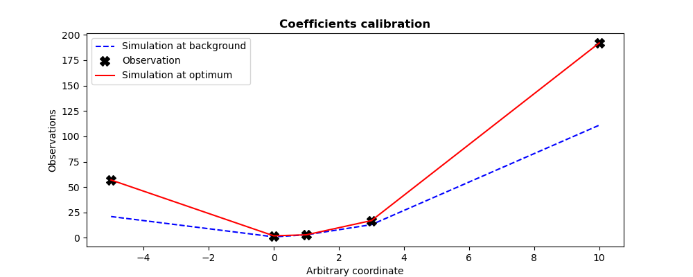
In the figure, the lines simply join the simulated values at the control points and make them easier to read.
We see, in this particularly simple case, that the optimum is identical to the
values of coefficients [2, -1, 2] used to generate the pseudo-observations
for the twin experiment. Naturally, the final simulation obtained with the
adjusted coefficients coincides with the observations at the 5 control points.
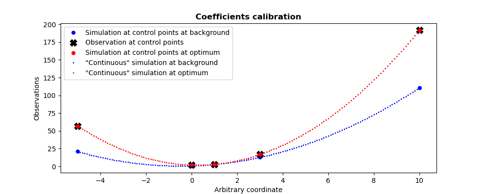
To illustrate more clearly the recalibration performed, using the same information, we can plot the “continuous” version of the quadratic curves available for the background state of the coefficients, and for the optimal state of the coefficients, together with the values obtained at the control points. In addition, to improve readability, the lines joining the simulations in the previous graph have been removed.
13.1.5.2. Second example
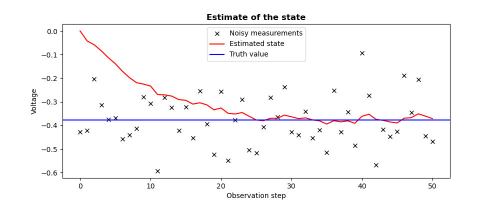
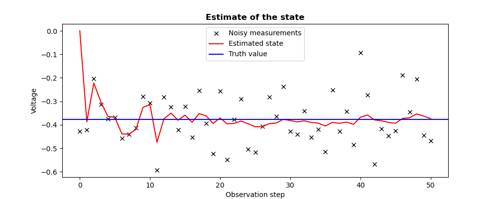
The 3DVAR can also be used for a time analysis of the observations of a given dynamic model. In this case, the analysis is performed iteratively, at the arrival of each observation. For this example, we use the same simple dynamic system [Welch06] that is analyzed in the Kalman Filter Python (TUI) use examples. For a good understanding of time management, please refer to the Timeline of steps for data assimilation operators in dynamics and the explanations in the section Going further in data assimilation for dynamics.
At each step, the classical 3DVAR analysis updates only the state of the system. By modifying the a priori covariance values with respect to the initial assumptions of the filtering, this 3DVAR reanalysis allows to converge towards the true trajectory, as illustrated in the associated figure, in a slightly slower speed than with a Kalman Filter.
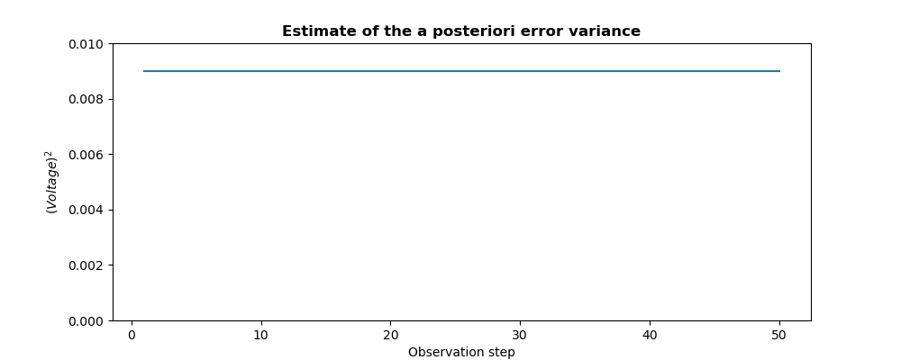
Note
Note about a posteriori covariances: classically, the 3DVAR iterative analysis updates only the state and not its covariance. As the assumptions of operators and a priori covariance remain unchanged here during the evolution, the a posteriori covariance is constant. The following plot of this a posteriori covariance allows us to insist on this property, which is entirely expected from the 3DVAR analysis. A more advanced hypothesis is proposed in the forthcoming example.
# -*- coding: utf-8 -*-
#
from numpy import array, random
random.seed(1234567)
Xtrue = -0.37727
Yobs = []
for i in range(51):
    Yobs.append([random.normal(Xtrue, 0.1, size=(1,)),])
#
print("Variational estimation of a time trajectory")
print("-------------------------------------------")
print("  Noisy measurements acquired on %i time steps"%(len(Yobs)-1,))
print("")
from adao import adaoBuilder
case = adaoBuilder.New()
#
case.setBackground         (Vector             = [0.])
case.setBackgroundError    (ScalarSparseMatrix = 0.1**2)
#
case.setObservationOperator(Matrix             = [1.])
case.setObservation        (VectorSerie        = Yobs)
case.setObservationError   (ScalarSparseMatrix = 0.3**2)
#
case.setEvolutionModel     (Matrix             = [1.])
case.setEvolutionError     (ScalarSparseMatrix = 1e-5)
#
case.setAlgorithmParameters(
    Algorithm="3DVAR",
    Parameters={
        "EstimationOf":"State",
        "StoreSupplementaryCalculations":[
            "Analysis",
            "APosterioriCovariance",
            ],
        },
    )
#
case.execute()
Xa = case.get("Analysis")
Pa = case.get("APosterioriCovariance")
#
print("  Analyzed state at final observation:", Xa[-1])
print("")
print("  Final a posteriori variance:", Pa[-1])
print("")
#
#-------------------------------------------------------------------------------
#
Observations = array([yo[0]   for yo in Yobs])
Estimates    = array([xa[0]   for xa in case.get("Analysis")])
Variances    = array([pa[0,0] for pa in case.get("APosterioriCovariance")])
#
import matplotlib.pyplot as plt
plt.rcParams["figure.figsize"] = (10, 4)
#
plt.figure()
plt.plot(Observations,"kx",label="Noisy measurements")
plt.plot(Estimates,"r-",label="Estimated state")
plt.axhline(Xtrue,color="b",label="Truth value")
plt.legend()
plt.title("Estimate of the state", fontweight="bold")
plt.xlabel("Observation step")
plt.ylabel("Voltage")
plt.savefig("simple_3DVAR2_state.png")
#
plt.figure()
iobs = range(1,len(Observations))
plt.plot(iobs,Variances[iobs],label="A posteriori error variance")
plt.title("Estimate of the a posteriori error variance", fontweight="bold")
plt.xlabel("Observation step")
plt.ylabel("$(Voltage)^2$")
plt.setp(plt.gca(),"ylim",[0,.01])
plt.savefig("simple_3DVAR2_variance.png")
The execution result is the following:
Variational estimation of a time trajectory
-------------------------------------------
  Noisy measurements acquired on 50 time steps

  Analyzed state at final observation: [-0.37110687]

  Final a posteriori variance: [[0.009]]
The figures illustrating the result of its execution are as follows:
13.1.5.3. Third example
From the preceding example, if one wants to adapt the time convergence of the 3DVAR, one can change, for example, the a priori covariance assumptions of the background errors during the iterations. This update is an assumption of the user, and there are multiple alternatives that will depend on the physics of the case. We illustrate one of them here.
We choose, in an arbitrary way, to make the a priori covariance of the
background errors to decrease by a constant factor  as long
as it remains above a limit value of
as long
as it remains above a limit value of  (which is the fixed
value of a priori covariance of the background errors of the previous
example), knowing that it starts at the value 1 (which is the fixed value of
a priori covariance of the background errors used for the first step of
Kalman filtering). This value is updated at each step, by re-injecting it as
the a priori covariance of the state which is used as a background in the
next step of analysis, in an explicit loop.
(which is the fixed
value of a priori covariance of the background errors of the previous
example), knowing that it starts at the value 1 (which is the fixed value of
a priori covariance of the background errors used for the first step of
Kalman filtering). This value is updated at each step, by re-injecting it as
the a priori covariance of the state which is used as a background in the
next step of analysis, in an explicit loop.
We notice in this case that the state estimation converges faster to the true value, and that the assimilation then behaves similarly to the examples for the Kalman Filter, or to the previous example with the manually adapted a priori covariances. Moreover, the a posteriori covariance decreases as long as we force the decrease of the a priori covariance.
Note
We insist on the fact that the a priori covariance variations, which determine the a posteriori covariance variations, are a user arbitrary assumption and not an obligation. This assumption must therefore be adapted to the physical case.
# -*- coding: utf-8 -*-
#
from numpy import array, random
random.seed(1234567)
Xtrue = -0.37727
Yobs = []
for i in range(51):
    Yobs.append([random.normal(Xtrue, 0.1, size=(1,)),])
#
print("Variational estimation of a time trajectory")
print("-------------------------------------------")
print("  Noisy measurements acquired on %i time steps"%(len(Yobs)-1,))
print("")
from adao import adaoBuilder
case = adaoBuilder.New()
#
case.setBackground         (Vector             = [0.])
#
case.setObservationOperator(Matrix             = [1.])
case.setObservationError   (ScalarSparseMatrix = 0.3**2)
#
case.setEvolutionModel     (Matrix             = [1.])
case.setEvolutionError     (ScalarSparseMatrix = 1e-5)
#
case.setAlgorithmParameters(
    Algorithm="3DVAR",
    Parameters={
        "EstimationOf":"State",
        "StoreSupplementaryCalculations":[
            "Analysis",
            "APosterioriCovariance",
            ],
        },
    )
#
# Loop to obtain an analysis at each observation arrival
#
Ca = 1.
for i in range(1,len(Yobs)):
    case.setObservation(Vector = Yobs[i])
    case.setBackgroundError(ScalarSparseMatrix = Ca) # Update of the covariance
    case.execute( nextStep = True )
    #
    # Hypothesis of the a priori covariance decay of the background error
    #
    if float(Ca) <= 0.1**2:
        Ca = 0.1**2
    else:
        Ca = Ca * 0.9**2
#
Xa = case.get("Analysis")
Pa = case.get("APosterioriCovariance")
#
print("  Analyzed state at final observation:", Xa[-1])
print("")
print("  Final a posteriori variance:", Pa[-1])
print("")
#
#-------------------------------------------------------------------------------
#
Observations = array([yo[0]   for yo in Yobs])
Estimates    = array([xa[0]   for xa in case.get("Analysis")])
Variances    = array([pa[0,0] for pa in case.get("APosterioriCovariance")])
#
import matplotlib.pyplot as plt
plt.rcParams["figure.figsize"] = (10, 4)
#
plt.figure()
plt.plot(Observations,"kx",label="Noisy measurements")
plt.plot(Estimates,"r-",label="Estimated state")
plt.axhline(Xtrue,color="b",label="Truth value")
plt.legend()
plt.title("Estimate of the state", fontweight="bold")
plt.xlabel("Observation step")
plt.ylabel("Voltage")
plt.savefig("simple_3DVAR3_state.png")
#
plt.figure()
iobs = range(1,len(Observations))
plt.plot(iobs,Variances[iobs],label="A posteriori error variance")
plt.title("Estimate of the a posteriori error variance", fontweight="bold")
plt.xlabel("Observation step")
plt.ylabel("$(Voltage)^2$")
plt.savefig("simple_3DVAR3_variance.png")
The execution result is the following:
Variational estimation of a time trajectory
-------------------------------------------
  Noisy measurements acquired on 50 time steps

  Analyzed state at final observation: [-0.37334336]

  Final a posteriori variance: [[0.009]]
The figures illustrating the result of its execution are as follows:

13.1.5.4. Correction by 3DVAR of the state of a Lorenz dynamic system
This example extends the simple use cases of the 3DVAR algorithm (see Examples with the “3DVAR”, or a similar example in [Asch16]). It describes the effect of data assimilation on the time forecast of a dynamic system. It is a highly simplified case that illustrates a classical approach in meteorology (short-term weather forecasting, below a two-week period) or in seasonal forecasting (longer-term weather forecasting, beyond a two-week period).
Here, we use a simple classical model of a dynamic system, named Lorenz
system, Lorenz oscillator, Lorenz3D or Lorenz63 after its author, the
mathematician and meteorologist Edward Lorenz ([Lorenz63], [WikipediaL63]).
It is available in integrated test models of ADAO under the name
Lorenz1963.
This three-dimensional nonlinear dynamical system is a highly simplified model of the Navier-Stokes equations, designed to study the coupling of atmosphere and ocean, in a particular physical convection configuration (Rayleigh-Bénard convection). It exhibits deterministic chaotic behavior, which means that the dynamical system is deterministic (from a continuous or discrete point of view), but its sensitivity to initial conditions or parameters enables an arbitrarily different trajectory to be obtained after a finite time for small variations in its initial conditions. This system is known as the origin of the concept of the butterfly effect [Butterfly72] and for its illustrative value.
This system depends on its initial conditions and on 3 physical parameters
 . The classical equations for state
 describing it are:
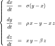
with time  , and with
  ,
,  ,
,
 current values of parameters characterizing a chaotic state.
The initial condition is arbitrary.
current values of parameters characterizing a chaotic state.
The initial condition is arbitrary.
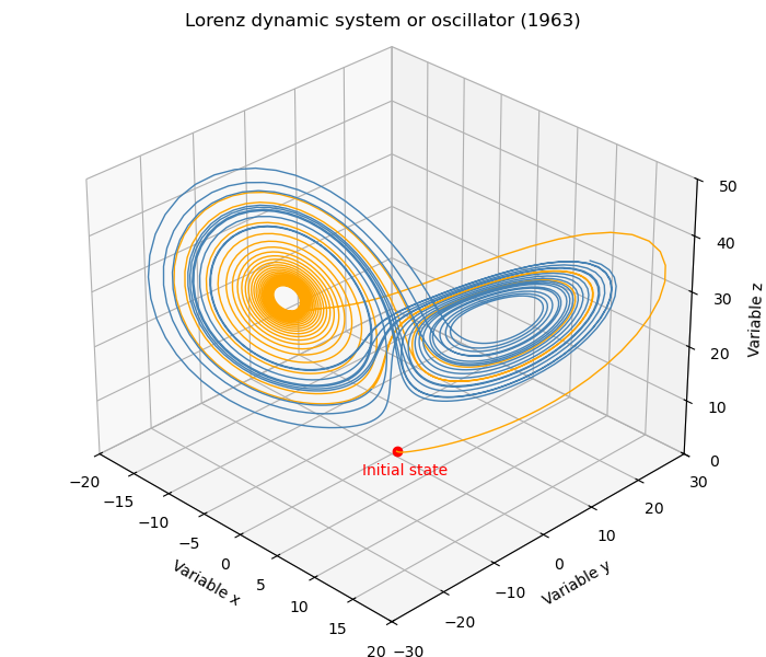
The following figure illustrates the Lorenz attractor by direct simulation of
this dynamic system, shown here for ![t\in[0,40]](_images/math/45fbba9c4d1e5ea67abce56103167e5906e9d7e9.png) and with initial
condition
and with initial
condition  . The attractor is the structure corresponding to the
long-term behavior of the Lorenz oscillator, which here appears as two
“butterfly wings”. The figure shows that the state variable
of this dynamical system evolves on a deterministic, non-periodic trajectory,
which wraps around one wing of the butterfly and then “jumps” to the other
wing, and so on in a seemingly erratic fashion. The figure below shows a single
trajectory, colored differently for its first and second halves to illustrate
the successive windings and jumps.
. The attractor is the structure corresponding to the
long-term behavior of the Lorenz oscillator, which here appears as two
“butterfly wings”. The figure shows that the state variable
of this dynamical system evolves on a deterministic, non-periodic trajectory,
which wraps around one wing of the butterfly and then “jumps” to the other
wing, and so on in a seemingly erratic fashion. The figure below shows a single
trajectory, colored differently for its first and second halves to illustrate
the successive windings and jumps.
If we observe the same trajectory by plotting the 3 components of the system
state separately (over a shorter period ![[0,10]](_images/math/847978eba481b018d604d0cde037d766a4ef2436.png) ), with the same
simulation parameters, we obtain the following figure:
), with the same
simulation parameters, we obtain the following figure:
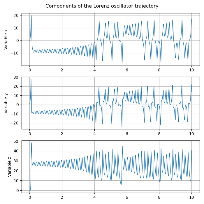
Noting that the amplitudes and temporal behaviors of the first two components
 and
and  are indeed not identical, despite their similarity,
this figure illustrates the property of chaos through an absence of spatial and
temporal regularity.
are indeed not identical, despite their similarity,
this figure illustrates the property of chaos through an absence of spatial and
temporal regularity.
To illustrate the analysis approach, we’ll be using twin experiments (see section To test a data assimilation chain: the twin experiments).
We choose here to perturb only the initial state of the simulation, using
the background value ![u^b=[2,3,4]](_images/math/7449e19c3c4a5e5a3520fa3440800c584402b549.png) , whose effects are to be compared with
those of the initial state, said to be ideal or true, unperturbed, equal to
, whose effects are to be compared with
those of the initial state, said to be ideal or true, unperturbed, equal to
![u^t=[1,1,1]](_images/math/3c1b0c54101eaee0392f5088dbd5e88dd1275d9c.png) .
.
The model is considered to be perfect, and is observed over the time interval
[0,2]. Pseudo-observations are of 10 in number,
constructed by sampling at time step  over this time
interval, based on a simulation from the initial unperturbed state
. To these exact sampled values is then added, on each
component, a Gaussian noise of amplitude
over this time
interval, based on a simulation from the initial unperturbed state
. To these exact sampled values is then added, on each
component, a Gaussian noise of amplitude  to obtain a
pseudo-observation. The order of magnitude of the noise is that of the
experimental noise of real variable measurements corresponding to the
simplified Lorenz model.
to obtain a
pseudo-observation. The order of magnitude of the noise is that of the
experimental noise of real variable measurements corresponding to the
simplified Lorenz model.
The following figure illustrates this information for the first variable (the others are similar), spread over the time interval [0,2] of measurement:
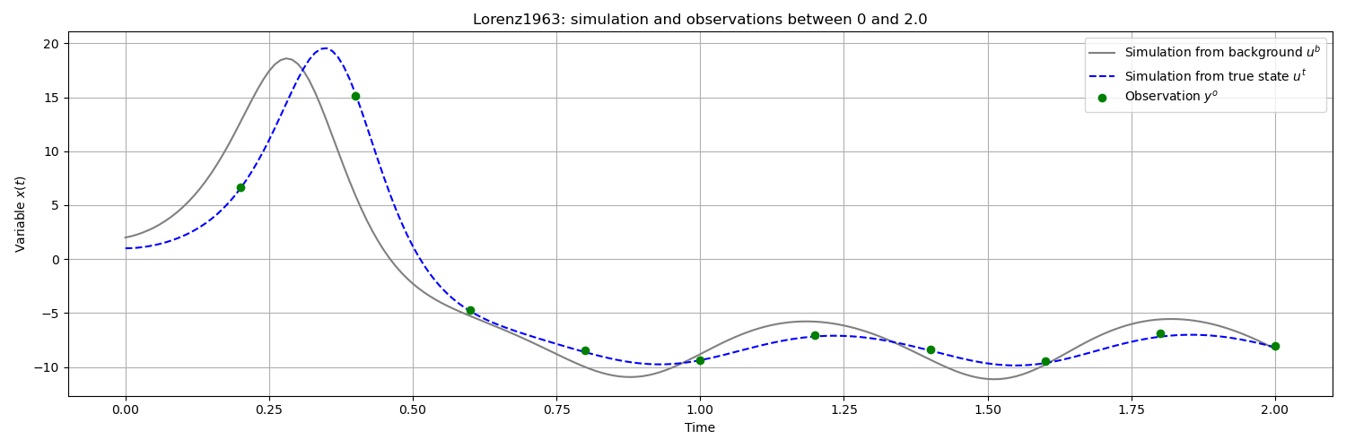
Note
It is strongly emphasized that successive observations are not available
simultaneously, at the initial time for example, but are available each
time the simulation reaches one of the measurement instants. It is also
recalled that the blue dashed simulation curve, obtained from the ideal or
true state , is unknown outside twin experiments. Only
trajectories plotted as continuous are known by simulation.
In numerical form, saved in a file named simple_3DVAR4Observations.csv to
be read, the observation values are as follows:
# Observations Lorenz1963 (format: t x y z)
#
0.20 +6.6255693323143952e+00 +1.3512204021575638e+01 +3.9860034533510582e+00
0.40 +1.5140047444332868e+01 +1.3495388075296226e+00 +4.6611660816669115e+01
0.60 -4.7609818075165542e+00 -7.9674154050023951e+00 +2.6781548199549242e+01
0.80 -8.4989430323515158e+00 -1.0087805440794597e+01 +2.5436627475898202e+01
1.00 -9.4032667798914851e+00 -8.4574726949541308e+00 +2.9469200645262447e+01
1.20 -7.0450610945351828e+00 -6.7568835708764148e+00 +2.6136357537101407e+01
1.40 -8.4087739643843644e+00 -9.7426531698975598e+00 +2.5181746694435667e+01
1.60 -9.4866303357699397e+00 -8.8142676152554458e+00 +2.9449435747857493e+01
1.80 -6.9109551287087747e+00 -6.3753292483483364e+00 +2.6504633755059768e+01
2.00 -8.0717069604712552e+00 -9.7394819137223507e+00 +2.4481237978123101e+01
Data assimilation is then used to correct the initial background trajectory of
the system with each new observation acquired. At each step  , the
current predicted state
, the
current predicted state  is modified to produce a new
analyzed state
is modified to produce a new
analyzed state  , taking into account this new
information
, taking into account this new
information  , then the simulation continues from this new
state. Assimilation of the observations is performed using the simple ADAO
script below. For better readability, the script explicitly presents the time
loop on the observations:
, then the simulation continues from this new
state. Assimilation of the observations is performed using the simple ADAO
script below. For better readability, the script explicitly presents the time
loop on the observations:
# -*- coding: utf-8 -*-
#
import numpy
from adao import adaoBuilder
from Models.Lorenz1963 import EDS as Lorenz1963
numpy.set_printoptions(precision=5)
#
u0Back = numpy.array([2, 3, 4])    # Background (not equal to the true state)
sigma_m = 0.15                     # Standard deviation of the measure noise
sigma_b = 0.1                      # Standard deviation of the background noise
H = numpy.eye(3)                   # Observation operator
ODE = Lorenz1963(dt = 0.01)        # Dynamic model
ODE.ObservationStep = 0.2          # Observation interval
#
observations = numpy.loadtxt("simple_3DVAR4Observations.csv")[:, 1:]
#
case = adaoBuilder.New()
case.setAlgorithmParameters(
    Algorithm="3DVAR",
    Parameters={"EstimationOf": "State"},
)
case.setBackground(Vector=u0Back)
case.setBackgroundError(ScalarSparseMatrix=sigma_b**2)
case.setObservationError(ScalarSparseMatrix=sigma_m**2)
case.setEvolutionError(ScalarSparseMatrix=1.0e-8)
case.setObservationOperator(Matrix=H)
#
print("Successive analysis correcting the forecasted state using the observation:")
for i in range(observations.shape[0]):
    case.setEvolutionModel(OneFunction=ODE.StateTransition)
    case.setObservation(Vector=observations[i, :])
    case.execute(nextStep=True)
    #
    Xa = case.get("Analysis")[-1]
    print(
        "  After observation nb %02i : Xa[%02i] = %+9.5f %+9.5f %+9.5f"
        % (i + 1, i + 1, Xa[0], Xa[1], Xa[2])
    )
The execution result is the following:
Successive analysis correcting the forecasted state using the observation:
  After observation nb 01 : Xa[01] = +10.81803 +20.13078 +12.79257
  After observation nb 02 : Xa[02] = +10.62741  -3.02604 +41.26296
  After observation nb 03 : Xa[03] =  -4.28903  -6.99542 +24.84772
  After observation nb 04 : Xa[04] =  -8.76412 -10.93891 +24.68112
  After observation nb 05 : Xa[05] =  -9.70093  -8.19724 +30.32881
  After observation nb 06 : Xa[06] =  -6.73955  -6.29483 +25.70542
  After observation nb 07 : Xa[07] =  -8.38183  -9.99790 +24.60690
  After observation nb 08 : Xa[08] =  -9.76835  -8.91467 +29.73469
  After observation nb 09 : Xa[09] =  -7.01017  -6.31548 +26.40657
  After observation nb 10 : Xa[10] =  -8.05253  -9.61682 +24.32317
The following figure illustrates, on the first variable, the forecasted, measured and analyzed states at each observation step, as well as the states simulated by the model between two observations. The temporal breaks in the trajectory are, by their very nature, the result of each assimilation operation with new observed information.
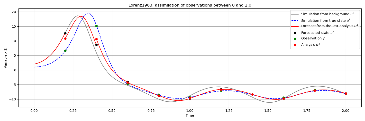
We can clearly see that the predicted state is more and
more consistent with each pseudo-observation , and that
each portion of the predicted trajectory is closer and closer to the unknown
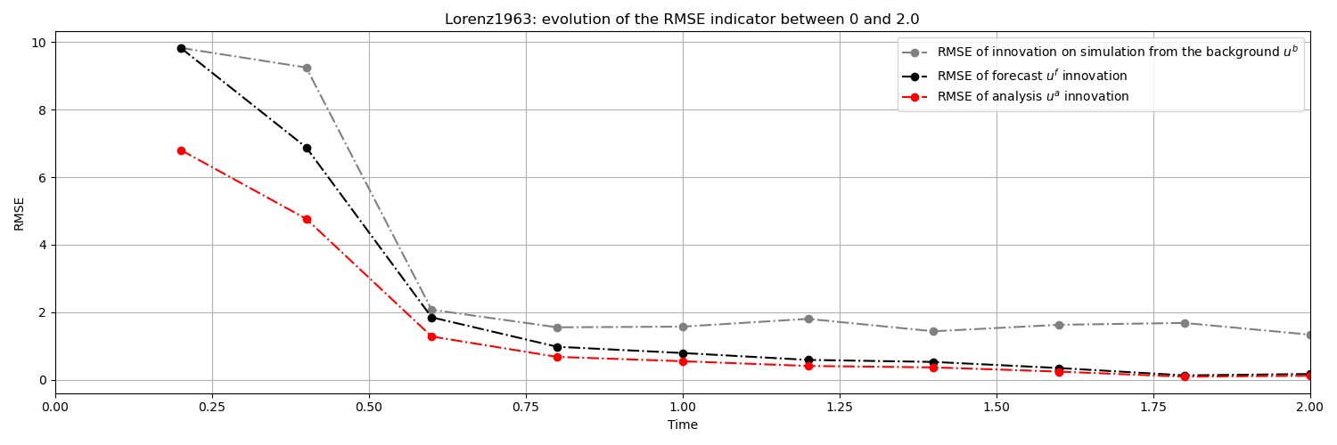
ideal trajectory resulting from the true state  . In the
following figure, the classical RMSE (Root-Mean-Square Error) measure of
deviations similarly describes this iterative improvement of forecasts and
analyses incorporating the information of observations.
. In the
following figure, the classical RMSE (Root-Mean-Square Error) measure of
deviations similarly describes this iterative improvement of forecasts and
analyses incorporating the information of observations.
It is also possible to compare the state forecasts obtained over the time
interval [2,10], which lies beyond the observation window concerned by the data
assimilation approach. There are three ways of establishing this temporal
simulation after the instant  :
:
we can calculate the forecast from the state at
, itself obtained
by simulation from the disturbed initial background state
at time  , in which only the background information is used;
we can calculate the forecast from the state at
, itself obtained
by simulation from the unperturbed initial state (ideal state or true
state) , which is considered the reference but known only
through the observations obtained from sampling with noise ;we can calculate the forecast resulting from data assimilation analysis, which comes from state correction by observations.
These three approaches are illustrated in the following figure, where the assimilation window is recalled over the time interval [0,2] and where forecasts are made over the time interval [2,10]:
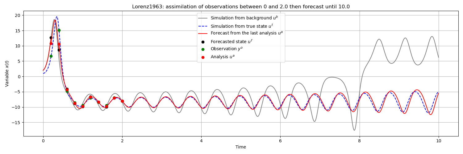
It is apparent that the forecast resulting from the  analysis, obtained by data assimilation at time , is much more in
line with the ideal simulation chosen for the twin
experiment, than the forecast resulting from the
analysis, obtained by data assimilation at time , is much more in
line with the ideal simulation chosen for the twin
experiment, than the forecast resulting from the  draft
simulated at . Even if the time extension of the simulation
necessarily leads to an increasing deviation from the true state, due to the
chaotic property of the Lorenz system, the correction by data assimilation
makes it possible to obtain an acceptable forecast over a much longer period of
time than the absence of correction intrinsically present in the background
simulation.
draft
simulated at . Even if the time extension of the simulation
necessarily leads to an increasing deviation from the true state, due to the
chaotic property of the Lorenz system, the correction by data assimilation
makes it possible to obtain an acceptable forecast over a much longer period of
time than the absence of correction intrinsically present in the background
simulation.