13.10. Calculation algorithm “KalmanFilter”¶

Description¶

This algorithm realizes an estimation of the state of a dynamic system by a Kalman Filter. In discrete form, it is an iterative (or recursive) estimator of the current state using the previous state and the current observations. The time (or pseudo-time) between two steps is the time between successive observations. Each iteration step is composed of two successive phases, classically called “prediction” and “correction”. The prediction step uses an incremental evolution operator to establish an estimate of the current state from the state estimated at the previous step. The correction (or update) step uses the current observations to improve the estimate by correcting the predicted state.

It is theoretically reserved for observation and incremental evolution operators cases which are linear, even if it sometimes works in “slightly” non-linear cases. One can verify the linearity of the operators with the help of a Checking algorithm “LinearityTest”.

Conceptually, we can represent the temporal pattern of action of the evolution and observation operators in this algorithm in the following way, with x the state, P the state error covariance, t the discrete iterative time :

Timeline of steps in Kalman filter data assimilation

In this scheme, the analysis (x,P) is obtained by means of the “correction” by observing the “prediction” of the previous state. We notice that there is no analysis performed at the initial time step (numbered 0 in the time indexing) because there is no forecast at this time (the background is stored as a pseudo analysis at the initial time step). If the observations are provided in series by the user, the first one is therefore not used.

This filter can also be used to estimate (jointly or solely) parameters and not the state, in which case neither the time nor the evolution have any meaning. The iteration steps are then linked to the insertion of a new observation in the recursive estimation. One should consult the section Going further in data assimilation for dynamics for the implementation concepts.

In case of non-linearity of the operators, even slightly marked, it will be preferred a Calculation algorithm “ExtendedKalmanFilter”, or a Calculation algorithm “UnscentedKalmanFilter” and a Calculation algorithm “UnscentedKalmanFilter” that are more powerful. One can verify the linearity of the operators with the help of a Checking algorithm “LinearityTest”.

Optional and required commands¶

The general required commands, available in the editing user graphical or textual interface, are the following:

Background: Vector. The variable indicates the background or initial vector used, previously noted as $\mathbf{x}^b$ . Its value is defined as a “Vector” or “VectorSerie” type object. Its availability in output is conditioned by the boolean “Stored” associated with input.

BackgroundError: Matrix. This indicates the background error covariance matrix, previously noted as $\mathbf{B}$ . Its value is defined as a “Matrix” type object, a “ScalarSparseMatrix” type object, or a “DiagonalSparseMatrix” type object, as described in detail in the section Requirements to describe covariance matrices. Its availability in output is conditioned by the boolean “Stored” associated with input.

EvolutionError: Matrix. The variable indicates the evolution error covariance matrix, usually noted as $\mathbf{Q}$ . It is defined as a “Matrix” type object, a “ScalarSparseMatrix” type object, or a “DiagonalSparseMatrix” type object, as described in detail in the section Requirements to describe covariance matrices. Its availability in output is conditioned by the boolean “Stored” associated with input.

EvolutionModel: Operator. The variable indicates the evolution model operator, usually noted $M$ , which describes an elementary step of evolution. Its value is defined as a “Function” type object or a “Matrix” type one. In the case of “Function” type, different functional forms can be used, as described in the section Requirements for functions describing an operator. If there is some control $U$ included in the evolution model, the operator has to be applied to a pair $(X,U)$ .

Observation: List of vectors. The variable indicates the observation vector used for data assimilation or optimization, and usually noted $\mathbf{y}^o$ . Its value is defined as an object of type “Vector” if it is a single observation (temporal or not) or “VectorSeries” if it is a succession of observations. Its availability in output is conditioned by the boolean “Stored” associated in input.

ObservationError: Matrix. The variable indicates the observation error covariance matrix, usually noted as $\mathbf{R}$ . It is defined as a “Matrix” type object, a “ScalarSparseMatrix” type object, or a “DiagonalSparseMatrix” type object, as described in detail in the section Requirements to describe covariance matrices. Its availability in output is conditioned by the boolean “Stored” associated with input.

ObservationOperator: Operator. The variable indicates the observation operator, usually noted as $H$ , which transforms the input parameters $\mathbf{x}$ to results $\mathbf{y}$ to be compared to observations $\mathbf{y}^o$ . Its value is defined as a “Function” type object or a “Matrix” type one. In the case of “Function” type, different functional forms can be used, as described in the section Requirements for functions describing an operator. If there is some control $U$ included in the observation, the operator has to be applied to a pair $(X,U)$ .

The general optional commands, available in the editing user graphical or textual interface, are indicated in List of commands and keywords for data assimilation or optimisation case. Moreover, the parameters of the command “AlgorithmParameters” allows to choose the specific options, described hereafter, of the algorithm. See Description of options of an algorithm by “AlgorithmParameters” for the good use of this command.

The options are the following:

EstimationOf

Predefined name. This key allows to choose the type of estimation to be performed. It can be either state-estimation, with a value of “State”, or parameter-estimation, with a value of “Parameters”. The default choice is “State”.

Example: {"EstimationOf":"Parameters"}

StoreSupplementaryCalculations

List of names. This list indicates the names of the supplementary variables, that can be available during or at the end of the algorithm, if they are initially required by the user. Their avalability involves, potentially, costly calculations or memory consumptions. The default is then a void list, none of these variables being calculated and stored by default (excepted the unconditionnal variables). The possible names are in the following list (the detailed description of each named variable is given in the following part of this specific algorithmic documentation, in the sub-section “Information and variables available at the end of the algorithm”): [ “Analysis”, “APosterioriCorrelations”, “APosterioriCovariance”, “APosterioriStandardDeviations”, “APosterioriVariances”, “BMA”, “CostFunctionJ”, “CostFunctionJAtCurrentOptimum”, “CostFunctionJb”, “CostFunctionJbAtCurrentOptimum”, “CostFunctionJo”, “CostFunctionJoAtCurrentOptimum”, “CurrentOptimum”, “CurrentState”, “CurrentStepNumber”, “ForecastCovariance”, “ForecastState”, “IndexOfOptimum”, “InnovationAtCurrentAnalysis”, “InnovationAtCurrentState”, “SimulatedObservationAtCurrentAnalysis”, “SimulatedObservationAtCurrentOptimum”, “SimulatedObservationAtCurrentState”, ].

Example : {"StoreSupplementaryCalculations":["BMA", "CurrentState"]}

Information and variables available at the end of the algorithm¶

At the output, after executing the algorithm, there are information and variables originating from the calculation. The description of Variables and informations available at the output show the way to obtain them by the method named get, of the variable “ADD” of the post-processing in graphical interface, or of the case in textual interface. The input variables, available to the user at the output in order to facilitate the writing of post-processing procedures, are described in the Inventory of potentially available information at the output.

Permanent outputs (non conditional)

The unconditional outputs of the algorithm are the following:

Analysis

List of vectors. Each element of this variable is an optimal state $\mathbf{x}^*$ in optimization or an analysis $\mathbf{x}^a$ in data assimilation.

Example: Xa = ADD.get("Analysis")[-1]

Set of on-demand outputs (conditional or not)

The whole set of algorithm outputs (conditional or not), sorted by alphabetical order, is the following:

Analysis

List of vectors. Each element of this variable is an optimal state $\mathbf{x}^*$ in optimization or an analysis $\mathbf{x}^a$ in data assimilation.

Example: Xa = ADD.get("Analysis")[-1]

APosterioriCorrelations

List of matrices. Each element is an a posteriori error correlations matrix of the optimal state, coming from the $\mathbf{A}$ covariance matrix. In order to get them, this a posteriori error covariances calculation has to be requested at the same time.

Example: C = ADD.get("APosterioriCorrelations")[-1]

APosterioriCovariance

List of matrices. Each element is an a posteriori error covariance matrix $\mathbf{A}$ of the optimal state.

Example: A = ADD.get("APosterioriCovariance")[-1]

APosterioriStandardDeviations

List of matrices. Each element is an a posteriori error standard errors diagonal matrix of the optimal state, coming from the $\mathbf{A}$ covariance matrix. In order to get them, this a posteriori error covariances calculation has to be requested at the same time.

Example: S = ADD.get("APosterioriStandardDeviations")[-1]

APosterioriVariances

List of matrices. Each element is an a posteriori error variance errors diagonal matrix of the optimal state, coming from the $\mathbf{A}$ covariance matrix. In order to get them, this a posteriori error covariances calculation has to be requested at the same time.

Example: V = ADD.get("APosterioriVariances")[-1]

BMA

List of vectors. Each element is a vector of difference between the background and the optimal state.

Example: bma = ADD.get("BMA")[-1]

CostFunctionJ

List of values. Each element is a value of the chosen error function $J$ .

Example: J = ADD.get("CostFunctionJ")[:]

CostFunctionJAtCurrentOptimum

List of values. Each element is a value of the error function $J$ . At each step, the value corresponds to the optimal state found from the beginning.

Example: JACO = ADD.get("CostFunctionJAtCurrentOptimum")[:]

CostFunctionJb

List of values. Each element is a value of the error function $J^b$ , that is of the background difference part. If this part does not exist in the error function, its value is zero.

Example: Jb = ADD.get("CostFunctionJb")[:]

CostFunctionJbAtCurrentOptimum

List of values. Each element is a value of the error function $J^b$ . At each step, the value corresponds to the optimal state found from the beginning. If this part does not exist in the error function, its value is zero.

Example: JbACO = ADD.get("CostFunctionJbAtCurrentOptimum")[:]

CostFunctionJo

List of values. Each element is a value of the error function $J^o$ , that is of the observation difference part.

Example: Jo = ADD.get("CostFunctionJo")[:]

CostFunctionJoAtCurrentOptimum

List of values. Each element is a value of the error function $J^o$ , that is of the observation difference part. At each step, the value corresponds to the optimal state found from the beginning.

Example: JoACO = ADD.get("CostFunctionJoAtCurrentOptimum")[:]

CurrentOptimum

List of vectors. Each element is the optimal state obtained at the usual step of the iterative algorithm procedure of the optimization algorithm. It is not necessarily the last state.

Example: Xo = ADD.get("CurrentOptimum")[:]

CurrentState

List of vectors. Each element is a usual state vector used during the iterative algorithm procedure.

Example: Xs = ADD.get("CurrentState")[:]

CurrentStepNumber

List of integers. Each element is the index of the current step in the iterative process, driven by the series of observations, of the algorithm used. This corresponds to the observation step used. Note: it is not the index of the current iteration of the algorithm even if it coincides for non-iterative algorithms.

Example: i = ADD.get("CurrentStepNumber")[-1]

ForecastCovariance

Liste of matrices. Each element is a forecast state error covariance matrix predicted by the model during the time iteration of the algorithm used.

Example : Pf = ADD.get("ForecastCovariance")[-1]

ForecastState

List of vectors. Each element is a state vector forecasted by the model during the iterative algorithm procedure.

Example: Xp = ADD.get("ForecastState")[:]

IndexOfOptimum

List of integers. Each element is the iteration index of the optimum obtained at the current step of the iterative algorithm procedure of the optimization algorithm. It is not necessarily the number of the last iteration.

Example: i = ADD.get("IndexOfOptimum")[-1]

InnovationAtCurrentAnalysis

List of vectors. Each element is an innovation vector at current analysis. This quantity is identical to the innovation vector at analysed state in the case of a single-state assimilation.

Example: ds = ADD.get("InnovationAtCurrentAnalysis")[-1]

InnovationAtCurrentState

List of vectors. Each element is an innovation vector at current state before analysis.

Example: ds = ADD.get("InnovationAtCurrentState")[-1]

SimulatedObservationAtCurrentAnalysis

List of vectors. Each element is an observed vector simulated by the observation operator from the current analysis, that is, in the observation space. This quantity is identical to the observed vector simulated at current state in the case of a single-state assimilation.

Example: hxs = ADD.get("SimulatedObservationAtCurrentAnalysis")[-1]

SimulatedObservationAtCurrentOptimum

List of vectors. Each element is a vector of observation simulated from the optimal state obtained at the current step the optimization algorithm, that is, in the observation space.

Example: hxo = ADD.get("SimulatedObservationAtCurrentOptimum")[-1]

SimulatedObservationAtCurrentState

List of vectors. Each element is an observed vector simulated by the observation operator from the current state, that is, in the observation space.

Example: hxs = ADD.get("SimulatedObservationAtCurrentState")[-1]

Python (TUI) use examples¶

Here is a very simple use of the given algorithm and its parameters, written in [DocR] Textual User Interface for ADAO (TUI/API), and from which input information allow to define an equivalent cas in graphical interface.

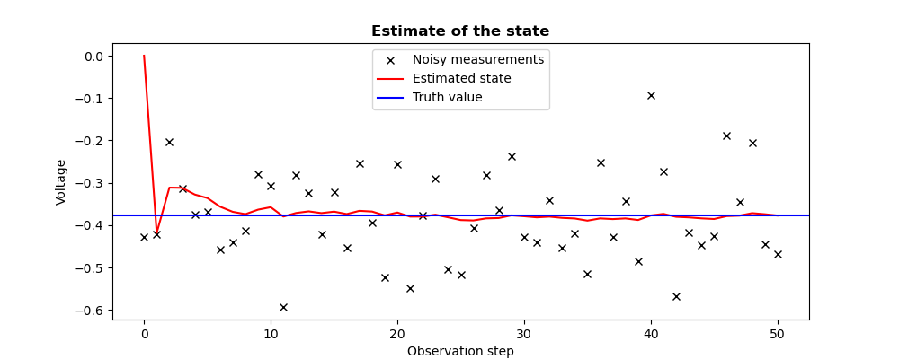
The Kalman Filter can be used for a reanalysis of observations of a given dynamical model. It is because the whole set of the observation full history is already known at the beginning of the time windows that it is called reanalysis, even if the iterative analysis keeps unkown the future observations at a given time step.

This example describes iterative estimation of a constant physical quantity (a voltage) following seminal example of [Welch06] (pages 11 and following, also available in the SciPy Cookbook). This model allows to illustrate the excellent behavior of this algorithm with respect to the measurement noise when the evolution model is simple. The physical problem is the estimation of the voltage, observed on 50 time steps, with noise, which imply 50 analysis steps by the filter. The idealized state (said the “true” value, unknown in a real case) is specified as Xtrue in the example. The observations $\mathbf{y}^o$ (denoted by Yobs in the example) are to be set, using the keyword “VectorSerie”, as a measure time series. We choose to emphasize the observations versus the background, by setting a great value for the background error variance with respect to the observation error variance. The first observation is not used because the background $\mathbf{x}^b$ is used as the first state estimate.

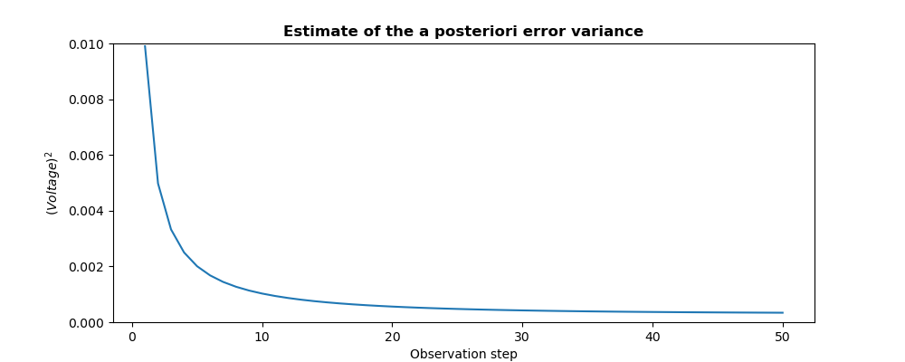
The adjustment is carried out by displaying intermediate results during iterative filtering. Using these intermediate results, one can also obtain figures that illustrate the state estimation and the associated a posteriori covariance estimation.

# -*- coding: utf-8 -*-
#
from numpy import array, random
random.seed(1234567)
Xtrue = -0.37727
Yobs = []
for i in range(51):
    Yobs.append([random.normal(Xtrue, 0.1, size=(1,)),])
#
print("Estimation of a constant variable by filtering")
print("----------------------------------------------")
print("  Noisy measurements acquired on %i time steps"%(len(Yobs)-1,))
print("")
from adao import adaoBuilder
case = adaoBuilder.New('')
#
case.setBackground         (Vector             = [0.])
case.setBackgroundError    (ScalarSparseMatrix = 1.)
#
case.setObservationOperator(Matrix             = [1.])
case.setObservation        (VectorSerie        = Yobs)
case.setObservationError   (ScalarSparseMatrix = 0.1**2)
#
case.setEvolutionModel     (Matrix             = [1.])
case.setEvolutionError     (ScalarSparseMatrix = 1e-5)
#
case.setAlgorithmParameters(
    Algorithm="KalmanFilter",
    Parameters={
        "StoreSupplementaryCalculations":[
            "Analysis",
            "APosterioriCovariance",
            ],
        },
    )
case.setObserver(
    Info="  Analyzed state at current observation:",
    Template='ValuePrinter',
    Variable='Analysis',
    )
#
case.execute()
Xa = case.get("Analysis")
Pa = case.get("APosterioriCovariance")
#
print("")
print("  Final a posteriori variance:",Pa[-1])
print("")
#
#-------------------------------------------------------------------------------
#
Observations = array([yo[0]   for yo in Yobs])
Estimates    = array([xa[0]   for xa in case.get("Analysis")])
Variances    = array([pa[0,0] for pa in case.get("APosterioriCovariance")])
#
import matplotlib.pyplot as plt
plt.rcParams['figure.figsize'] = (10, 4)
#
plt.figure()
plt.plot(Observations,'kx',label='Noisy measurements')
plt.plot(Estimates,'r-',label='Estimated state')
plt.axhline(Xtrue,color='b',label='Truth value')
plt.legend()
plt.title('Estimate of the state', fontweight='bold')
plt.xlabel('Observation step')
plt.ylabel('Voltage')
plt.savefig("simple_KalmanFilter1_state.png")
#
plt.figure()
iobs = range(1,len(Observations))
plt.plot(iobs,Variances[iobs],label='A posteriori error variance')
plt.title('Estimate of the a posteriori error variance', fontweight='bold')
plt.xlabel('Observation step')
plt.ylabel('$(Voltage)^2$')
plt.setp(plt.gca(),'ylim',[0,.01])
plt.savefig("simple_KalmanFilter1_variance.png")

The execution result is the following:

Estimation of a constant variable by filtering
----------------------------------------------
  Noisy measurements acquired on 50 time steps

  Analyzed state at current observation: [0.]
  Analyzed state at current observation: [-0.41804504]
  Analyzed state at current observation: [-0.3114053]
  Analyzed state at current observation: [-0.31191336]
  Analyzed state at current observation: [-0.32761493]
  Analyzed state at current observation: [-0.33597167]
  Analyzed state at current observation: [-0.35629573]
  Analyzed state at current observation: [-0.36840289]
  Analyzed state at current observation: [-0.37392713]
  Analyzed state at current observation: [-0.36331937]
  Analyzed state at current observation: [-0.35750362]
  Analyzed state at current observation: [-0.37963052]
  Analyzed state at current observation: [-0.37117993]
  Analyzed state at current observation: [-0.36732985]
  Analyzed state at current observation: [-0.37148382]
  Analyzed state at current observation: [-0.36798059]
  Analyzed state at current observation: [-0.37371077]
  Analyzed state at current observation: [-0.3661228]
  Analyzed state at current observation: [-0.36777529]
  Analyzed state at current observation: [-0.37681677]
  Analyzed state at current observation: [-0.37007654]
  Analyzed state at current observation: [-0.37974517]
  Analyzed state at current observation: [-0.37964703]
  Analyzed state at current observation: [-0.37514278]
  Analyzed state at current observation: [-0.38143128]
  Analyzed state at current observation: [-0.38790654]
  Analyzed state at current observation: [-0.38880008]
  Analyzed state at current observation: [-0.38393577]
  Analyzed state at current observation: [-0.3831028]
  Analyzed state at current observation: [-0.37680097]
  Analyzed state at current observation: [-0.37891813]
  Analyzed state at current observation: [-0.38147782]
  Analyzed state at current observation: [-0.37981569]
  Analyzed state at current observation: [-0.38274266]
  Analyzed state at current observation: [-0.38418507]
  Analyzed state at current observation: [-0.38923054]
  Analyzed state at current observation: [-0.38400006]
  Analyzed state at current observation: [-0.38562502]
  Analyzed state at current observation: [-0.3840503]
  Analyzed state at current observation: [-0.38775222]
  Analyzed state at current observation: [-0.37700787]
  Analyzed state at current observation: [-0.37328191]
  Analyzed state at current observation: [-0.38024181]
  Analyzed state at current observation: [-0.3815806]
  Analyzed state at current observation: [-0.38392063]
  Analyzed state at current observation: [-0.38539266]
  Analyzed state at current observation: [-0.37856929]
  Analyzed state at current observation: [-0.37744505]
  Analyzed state at current observation: [-0.37154554]
  Analyzed state at current observation: [-0.37405773]
  Analyzed state at current observation: [-0.37725236]

  Final a posteriori variance: [[0.00033921]]

The figures illustrating the result of its execution are as follows:

_images/simple_KalmanFilter1_variance.png

The Kalman filter can also be used for a running analysis of the observations of a given dynamic model. In this case, the analysis is conducted iteratively, at the arrival of each observation.

The following example deals with the same simple dynamic system from the reference [Welch06]. The essential difference consists in carrying out the execution of a Kalman step at the arrival of each observation provided iteratively. The keyword “nextStep”, included in the execution order, allows to not store the background in duplicate of the previous analysis.

In an entirely similar way to the reanalysis (knowing that intermediate results can be displayed, which are omitted here for simplicity), estimation gives the same results during iterative filtering. Thanks to these intermediate information, one can also obtain the graphs illustrating the estimation of the state and the associated a posteriori error covariance.

# -*- coding: utf-8 -*-
#
from numpy import array, random
random.seed(1234567)
Xtrue = -0.37727
Yobs = []
for i in range(51):
    Yobs.append([random.normal(Xtrue, 0.1, size=(1,)),])
#
print("Estimation of a constant variable by filtering")
print("----------------------------------------------")
print("  Noisy measurements acquired on %i time steps"%(len(Yobs)-1,))
print("")
from adao import adaoBuilder
case = adaoBuilder.New('')
#
case.setBackground         (Vector             = [0.])
case.setBackgroundError    (ScalarSparseMatrix = 1.)
#
case.setObservationOperator(Matrix             = [1.])
case.setObservationError   (ScalarSparseMatrix = 0.1**2)
#
case.setEvolutionModel     (Matrix             = [1.])
case.setEvolutionError     (ScalarSparseMatrix = 1e-5)
#
case.setAlgorithmParameters(
    Algorithm="KalmanFilter",
    Parameters={
        "StoreSupplementaryCalculations":[
            "Analysis",
            "APosterioriCovariance",
            ],
        },
    )
#
# Loop to obtain an analysis at each observation arrival
#
for i in range(1,len(Yobs)):
    case.setObservation(Vector = Yobs[i])
    case.execute( nextStep = True )
#
Xa = case.get("Analysis")
Pa = case.get("APosterioriCovariance")
#
print("  Analyzed state at final observation:", Xa[-1])
print("")
print("  Final a posteriori variance:", Pa[-1])
print("")
#
#-------------------------------------------------------------------------------
#
Observations = array([yo[0]   for yo in Yobs])
Estimates    = array([xa[0]   for xa in case.get("Analysis")])
Variances    = array([pa[0,0] for pa in case.get("APosterioriCovariance")])
#
import matplotlib.pyplot as plt
plt.rcParams['figure.figsize'] = (10, 4)
#
plt.figure()
plt.plot(Observations,'kx',label='Noisy measurements')
plt.plot(Estimates,'r-',label='Estimated state')
plt.axhline(Xtrue,color='b',label='Truth value')
plt.legend()
plt.title('Estimate of the state', fontweight='bold')
plt.xlabel('Observation step')
plt.ylabel('Voltage')
plt.savefig("simple_KalmanFilter2_state.png")
#
plt.figure()
iobs = range(1,len(Observations))
plt.plot(iobs,Variances[iobs],label='A posteriori error variance')
plt.title('Estimate of the a posteriori error variance', fontweight='bold')
plt.xlabel('Observation step')
plt.ylabel('$(Voltage)^2$')
plt.setp(plt.gca(),'ylim',[0,.01])
plt.savefig("simple_KalmanFilter2_variance.png")